Maxwell's Equations and Vector Potentials


02/13/2017
PHY 712 Spring 2017 -- Lecture 14
1
P
H
Y
7
1
2
E
l
e
c
t
r
o
d
y
n
a
m
i
c
s
9
-
9
:
5
0
A
M
M
W
F
O
l
i
n
1
0
3
P
l
a
n
f
o
r
L
e
c
t
u
r
e
1
4
:
S
t
a
r
t
r
e
a
d
i
n
g
C
h
a
p
t
e
r
6
1.
M
a
x
w
e
l
l
’
s
f
u
l
l
e
q
u
a
t
i
o
n
s
;
e
f
f
e
c
t
s
o
f
t
i
m
e
v
a
r
y
i
n
g
f
i
e
l
d
s
a
n
d
s
o
u
r
c
e
s
2.
G
a
u
g
e
c
h
o
i
c
e
s
a
n
d
t
r
a
n
s
f
o
r
m
a
t
i
o
n
s
3.
G
r
e
e
n
’
s
f
u
n
c
t
i
o
n
f
o
r
v
e
c
t
o
r
a
n
d
s
c
a
l
a
r
p
o
t
e
n
t
i
a
l
s

02/13/2017
PHY 712 Spring 2017 -- Lecture 14
2

02/13/2017
PHY 712 Spring 2017 -- Lecture 14
3
Full electrodynamics with time varying fields and sources
http://www.clerkmaxwellfoundation.org/
Image of statue of
James Clerk-Maxwell
in Edinburgh
"
F
r
o
m
a
l
o
n
g
v
i
e
w
o
f
t
h
e
h
i
s
t
o
r
y
o
f
m
a
n
k
i
n
d
-
s
e
e
n
f
r
o
m
,
s
a
y
,
t
e
n
t
h
o
u
s
a
n
d
y
e
a
r
s
f
r
o
m
n
o
w
-
t
h
e
r
e
c
a
n
b
e
l
i
t
t
l
e
d
o
u
b
t
t
h
a
t
t
h
e
m
o
s
t
s
i
g
n
i
f
i
c
a
n
t
e
v
e
n
t
o
f
t
h
e
1
9
t
h
c
e
n
t
u
r
y
w
i
l
l
b
e
j
u
d
g
e
d
a
s
M
a
x
w
e
l
l
'
s
d
i
s
c
o
v
e
r
y
o
f
t
h
e
l
a
w
s
o
f
e
l
e
c
t
r
o
d
y
n
a
m
i
c
s
"
Richard P Feynman
02/13/2017
PHY 712 Spring 2017 -- Lecture 14
4
02/13/2017
PHY 712 Spring 2017 -- Lecture 14
5
02/13/2017
PHY 712 Spring 2017 -- Lecture 14
6
Formulation of Maxwell’s equations in terms of vector and
scalar potentials
02/13/2017
PHY 712 Spring 2017 -- Lecture 14
7
Formulation of Maxwell’s equations in terms of vector and
scalar potentials -- continued
02/13/2017
PHY 712 Spring 2017 -- Lecture 14
8
Formulation of Maxwell’s equations in terms of vector and
scalar potentials -- continued
02/13/2017
PHY 712 Spring 2017 -- Lecture 14
9
Formulation of Maxwell’s equations in terms of vector and
scalar potentials -- continued
02/13/2017
PHY 712 Spring 2017 -- Lecture 14
10
Formulation of Maxwell’s equations in terms of vector and
scalar potentials -- continued
02/13/2017
PHY 712 Spring 2017 -- Lecture 14
11
Formulation of Maxwell’s equations in terms of vector and
scalar potentials -- continued
02/13/2017
PHY 712 Spring 2017 -- Lecture 14
12
Solution of Maxwell’s equations in the Lorentz gauge
02/13/2017
PHY 712 Spring 2017 -- Lecture 14
13
Solution of Maxwell’s equations in the Lorentz gauge -- continued
02/13/2017
PHY 712 Spring 2017 -- Lecture 14
14
Solution of Maxwell’s equations in the Lorentz gauge -- continued
02/13/2017
PHY 712 Spring 2017 -- Lecture 14
15
Solution of Maxwell’s equations in the Lorentz gauge -- continued
02/13/2017
PHY 712 Spring 2017 -- Lecture 14
16
Solution of Maxwell’s equations in the Lorentz gauge -- continued
02/13/2017
PHY 712 Spring 2017 -- Lecture 14
17
Solution of Maxwell’s equations in the Lorentz gauge -- continued
02/13/2017
PHY 712 Spring 2017 -- Lecture 14
18
Solution of Maxwell’s equations in the Lorentz gauge -- continued
02/13/2017
PHY 712 Spring 2017 -- Lecture 14
19
Solution of Maxwell’s equations in the Lorentz gauge -- continued
Liènard-Wiechert potentials and fields --
D
e
t
e
r
m
i
n
a
t
i
o
n
o
f
t
h
e
s
c
a
l
a
r
a
n
d
v
e
c
t
o
r
p
o
t
e
n
t
i
a
l
s
f
o
r
a
m
o
v
i
n
g
p
o
i
n
t
p
a
r
t
i
c
l
e
(
a
l
s
o
s
e
e
L
a
n
d
a
u
a
n
d
L
i
f
s
h
i
t
z
T
h
e
C
l
a
s
s
i
c
a
l
T
h
e
o
r
y
o
f
F
i
e
l
d
s
,
C
h
a
p
t
e
r
8
.
)
Consider the fields produced by the following source: a point
charge
q
moving on a trajectory
R
q
(t)
.
q
R
q
(t)
02/13/2017
PHY 712 Spring 2017 -- Lecture 14
20
Solution of Maxwell’s equations in the Lorentz gauge -- continued
We performing the integrations over first
d
3
r’
and then
dt’
making use of the fact that for any function of
t’
,
where the ``retarded time'' is defined to be
02/13/2017
PHY 712 Spring 2017 -- Lecture 14
21
Solution of Maxwell’s equations in the Lorentz gauge -- continued
Resulting scalar and vector potentials:
Notation:
02/13/2017
PHY 712 Spring 2017 -- Lecture 14
22
Comment on Lienard-Wiechert potential results
02/13/2017
PHY 712 Spring 2017 -- Lecture 14
23
Comment on Lienard-Wiechert potential results -- continued
02/13/2017
PHY 712 Spring 2017 -- Lecture 14
24
Summary of results for fields due to moving charge –
Li
é
nard Wiechert potentials
Resulting scalar and vector potentials:
Notation:
Significance of Maxwell's full equations, effects of time-varying fields and sources, gauge choices, Green's function for vector and scalar potentials, and formulation of Maxwell's equations in terms of vector and scalar potentials. Delve into the essence of electromagnetism with detailed insights into the historical impact and theoretical foundations provided by Maxwell's discoveries.

Uploaded on Feb 25, 2025 | 0 Views
Download Presentation

Please find below an Image/Link to download the presentation.
The content on the website is provided AS IS for your information and personal use only. It may not be sold, licensed, or shared on other websites without obtaining consent from the author.If you encounter any issues during the download, it is possible that the publisher has removed the file from their server.
You are allowed to download the files provided on this website for personal or commercial use, subject to the condition that they are used lawfully. All files are the property of their respective owners.
The content on the website is provided AS IS for your information and personal use only. It may not be sold, licensed, or shared on other websites without obtaining consent from the author.
E N D
Presentation Transcript
PHY 712 Electrodynamics 9-9:50 AM MWF Olin 103 Plan for Lecture 14: Start reading Chapter 6 1. Maxwell s full equations; effects of time varying fields and sources 2. Gauge choices and transformations 3. Green s function for vector and scalar potentials 02/13/2017 PHY 712 Spring 2017 -- Lecture 14 1
02/13/2017 PHY 712 Spring 2017 -- Lecture 14 2
Full electrodynamics with time varying fields and sources "From a long view of the history of mankind - seen from, say, ten thousand years from now - there can be little doubt that the most significant event of the 19th century will be judged as Maxwell's discovery of the laws of electrodynamics" Image of statue of James Clerk-Maxwell in Edinburgh Richard P Feynman http://www.clerkmaxwellfoundation.org/ 02/13/2017 PHY 712 Spring 2017 -- Lecture 14 3
= D Coulomb' law s : free D t = H J Ampere - Maxwell' law s : free B t + = E Faraday' law s : 0 = B magnetic No monopoles : 0 02/13/2017 PHY 712 Spring 2017 -- Lecture 14 4
= = P M Microscopi or vacuum c form ( E 0; 0) : = Coulomb' law s : / 0 E 1 c = B J Ampere - Maxwell' law s : 0 2 t B + = E Faraday' law s : 0 t = B magnetic No monopoles : 0 1 = 2 c 0 0 02/13/2017 PHY 712 Spring 2017 -- Lecture 14 5
Formulation of Maxwells equations in terms of vector and scalar potentials = = B B A 0 B A + = + = E E 0 0 t t A + = E t A = E or t 02/13/2017 PHY 712 Spring 2017 -- Lecture 14 6
Formulation of Maxwells equations in terms of vector and scalar potentials -- continued = E / : 0 ( ) t A = 2 / 0 E t 1 c = B J 0 2 ( ) t 2 A 2 t 1 c ( ) + + = A J 0 2 02/13/2017 PHY 712 Spring 2017 -- Lecture 14 7
Formulation of Maxwells equations in terms of vector and scalar potentials -- continued General form for the scalar and vector potential equations: = + + ( ) A 2 / 0 t ( ) 2 A 1 c ( ) = A J 0 2 2 t t = A Coulomb gauge form -- require = + = J J 0 C 2 / 0 C ( ) 2 A 1 c 1 c + = C 2 A J C 0 C 2 2 2 t t + = = J with t J J Note that 0 and 0 l l t 02/13/2017 PHY 712 Spring 2017 -- Lecture 14 8
Formulation of Maxwells equations in terms of vector and scalar potentials -- continued require - - form gauge Coulomb + = A 0 C = 2 / 0 C ( ) 2 A 1 1 + = 2 A J C C 0 C 2 2 2 c J t c t = + = = J J J J Note that with and 0 0 l t l t Continuity + equation for charge = current and density : ( ) = = J J 0 C 0 l l t t t ( ) ( ) 1 = = J C C 0 0 0 l 2 c t t 2 A 1 + = 2 A J C 0 C t 2 2 c t 02/13/2017 PHY 712 Spring 2017 -- Lecture 14 9
Formulation of Maxwells equations in terms of vector and scalar potentials -- continued Review of the general equations: = + + ( ) A 2 / 0 t ( ) 2 A 1 c ( ) = A J 0 2 2 t t 1 c + = A Lorentz gauge form -- require 0 L L 2 t 2 1 c + = 2 / L 0 L 2 2 t A 2 1 c + = 2 A J L 0 L 2 2 t 02/13/2017 PHY 712 Spring 2017 -- Lecture 14 10
Formulation of Maxwells equations in terms of vector and scalar potentials -- continued 1 c + = A require - - form gauge Lorentz 0 L L 2 t t A 2 1 c + = 2 / L 0 L 2 2 2 1 c + = 2 A J L 0 L 2 2 t t = + and = A A Alternate potentials : ' ' L L L L t 2 1 c = 2 Yields same physics provided that : 0 2 2 02/13/2017 PHY 712 Spring 2017 -- Lecture 14 11
Solution of Maxwells equations in the Lorentz gauge 1 0 2 2 = t c A A 2 2 / L L 2 1 c = 2 J L 0 L 2 2 t Consider t general he t form of the 3 - dimensiona wave l equation : 2 1 c = 2 4 f 2 2 ( ) ( ) wave source r r , field , t f t 02/13/2017 PHY 712 Spring 2017 -- Lecture 14 12
Solution of Maxwells equations in the Lorentz gauge -- continued represent , Let , , x y z A A A Let represent , , , f J J J x y z ( t ) 2 r 1 c , t ( ) ( ) = 2 r r , 4 , t f t 2 2 Green' function s : 2 1 c ( ) ( ) ( ) = 2 3 r ' , ' r r r , ; 4 ' ' G t t t t 2 2 t ( ) r Formal solution for field , : t ( ) ( ) ( ) ( f ) = + 3 r r r ' , ' r ' , ' r , , ' ' G , ; t t d r dt t t t = 0 f 02/13/2017 PHY 712 Spring 2017 -- Lecture 14 13
Solution of Maxwells equations in the Lorentz gauge -- continued Determinat ion of the form for the Green' function s : 2 1 c ( ) ( ) ( ) = 2 3 r ' , ' r r r , ; 4 ' ' G t t t t 2 2 t For the case of isotropic boundary v infinity at alues : 1 1 c ( ) = r ' , ' r r r , ; ' ' G t t t t r r ' ( ) r Formal solution t r = for field t r , : t ( ) ( ) + , , = 0 f 1 1 c ( ) 3 r r ' , ' r ' ' ' ' d r dt t t f t r r ' 02/13/2017 PHY 712 Spring 2017 -- Lecture 14 14
Solution of Maxwells equations in the Lorentz gauge -- continued Analysis of the Green's function: 2 1 c ( ) ( ) ( ) = 2 3 r , ; ', ' t r r r 4 ' ' G t t t 2 2 t "Proof" -- Fourier analysis in the time domain -- note that 1 ( ) ( ) t t ' i = ' t t d e 2 Define: 1 ( ) ( ) ( ) t t ' i = r , ; ', ' t r , ', r r G t d e G 2 2 ( ) ( ) + = 2 3 , ', r r r r 4 ' G 2 c 02/13/2017 PHY 712 Spring 2017 -- Lecture 14 15
Solution of Maxwells equations in the Lorentz gauge -- continued Analysis of the Green' function s (continued : ) 2 ~ ( ) ( ) + = 2 3 r , ' r r r , 4 ' G 2 c case For the of = isotropic r boundary v r infinity at alues : ~ ~ ( ) ( ) ( r , ' r , ' r , G G ~ ) is , ' r r r Further assuming that isotropic in ' : G R 2 2 1 ~ d ( ) ( ) + = 3 r , ' r r r , 4 ' R G 2 2 R dR c 1 ~ ( ) = / i R c r , ' r Solution : , G e R 02/13/2017 PHY 712 Spring 2017 -- Lecture 14 16
Solution of Maxwells equations in the Lorentz gauge -- continued function s Green' the of Analysis (continued : ) 1 ~ ( ) r / ' r i c = r , ' r , G e r r ' 1 ~ ( ) ( ) ( ) = ' i t t r ' , ' r r , ' r , ; e G , G t t d 2 1 1 ( ) r / ' r i c = ' i t t e d e r r 2 ' 1 1 ( ) r / ' r ' i t t c = e d r r ' 2 1 1 ( ) ( ) c = = r / ' r r / ' r ' ' t t c t t r r r r ' ' 02/13/2017 PHY 712 Spring 2017 -- Lecture 14 17
Solution of Maxwells equations in the Lorentz gauge -- continued 1 ( ( ) ) ( ) = r ' , ' r r / ' r , ; ' G t t t t c r r ' ( ) + r Solution for t field = , : t ( ) ( ) r r , , t = 0 f 1 1 c ( ) 3 r r ' , ' r ' ' ' ' d r dt t t f t r r ' 02/13/2017 PHY 712 Spring 2017 -- Lecture 14 18
Solution of Maxwells equations in the Lorentz gauge -- continued Li nard-Wiechert potentials and fields -- Determination of the scalar and vector potentials for a moving point particle (also see Landau and Lifshitz The Classical Theory of Fields, Chapter 8.) Consider the fields produced by the following source: a point charge q moving on a trajectory Rq(t). = 3 r r R Charge density: ( , ) t ( ( )) t q q R ( ) t d . q = 3 J r R r R R Current density: ( , ) ( ) t ( ( )), where t ( ) t . t q q q q dt Rq(t) q 02/13/2017 PHY 712 Spring 2017 -- Lecture 14 19
Solution of Maxwells equations in the Lorentz gauge -- continued ( , ' ') r r r 1 t ( ) = 3 ( , ) r r r d r dt ' ' ' ( | ' | / ) c t t t 4 | '] | 0 J r 1 ( ',t') r r ( ) = ' ( 3 ( , ) A r r r d r dt ' ' | '| / ) . c t t t 2 4 | '| c 0 We performing the integrations over first d3r and then dt making use of the fact that for any function of t , ( ( ) ( | ( )| / ) ' ' ' q d f t t t t t ( ) r f t r ) = r R ' , c R r R R ( ) ( | c ( )) )| t t q r q r 1 ( t q r where the ``retarded time'' is defined to be | r t t r R ( )|. t q r c 02/13/2017 PHY 712 Spring 2017 -- Lecture 14 20
Solution of Maxwells equations in the Lorentz gauge -- continued Resulting scalar and vector potentials: 1 q = ( , ) r , t v R 4 R 0 c v v R q = A ( , r ) , t 2 4 c R 0 c Notation: R r R ( ) rt r R | ( )|. t q q r t t r v R c ( ), rt q 02/13/2017 PHY 712 Spring 2017 -- Lecture 14 21
Comment on Lienard-Wiechert potential results function any for that Note : F(x) Now = ( ) ( ) ( ) F x x x dx F x 0 0 - = = consider function a for which , for 0 , 2 , 1 p(x) p(x ) i i dp ( ) i - - = ( ) ( ( )) ( ) F x p x dx F x x x dx x i dx x i ( ) F i = i dp dx x i 02/13/2017 PHY 712 Spring 2017 -- Lecture 14 22
Comment on Lienard-Wiechert potential results -- continued ( ) ( R f t ( ) = r In this case we have: ( ') f t ( ') p t ' dt ) ( ) r t c ( ) t R r R ' - q q 1 ( ) r t r q ( ) t r R ' q where: ( ') ' p t t t c ( ) ' c R ' d t ( ) ( ) t ( ) q r R ( ) t c ( ) t ' R r R ' ' ( ') ' dt dp t q dt q q = 1 1 ( ) t ( ) t r R r R ' ' q q 02/13/2017 PHY 712 Spring 2017 -- Lecture 14 23
Summary of results for fields due to moving charge Li nard Wiechert potentials Resulting scalar and vector potentials: 1 q = ( , ) r , t v R 4 R 0 c v v R q = A ( , r ) , t 2 4 c R 0 c Notation: R r R ( ) rt r R | ( )|. t q q r t t r v R c ( ), rt q 02/13/2017 PHY 712 Spring 2017 -- Lecture 14 24