Lecture on Hashing and Data Structures
Explore the principles of imperative computation through a lecture on hashing, dictionaries, sets, and hash tables. Understand the use of arrays for collections and mappings, and delve into dictionaries beyond arrays. Discover main operations and functionalities associated with arrays and dictionaries in computer science.

Download Presentation

Please find below an Image/Link to download the presentation.
The content on the website is provided AS IS for your information and personal use only. It may not be sold, licensed, or shared on other websites without obtaining consent from the author. If you encounter any issues during the download, it is possible that the publisher has removed the file from their server.
You are allowed to download the files provided on this website for personal or commercial use, subject to the condition that they are used lawfully. All files are the property of their respective owners.
The content on the website is provided AS IS for your information and personal use only. It may not be sold, licensed, or shared on other websites without obtaining consent from the author.
E N D
Presentation Transcript
15-122: Principles of Imperative Computation Lecture 13: Hashing March 03, 2024
Today Last lecture: Unbounded arrays Today s lecture: Dictionaries, sets, and hash tables Announcements: Written assignment 7 is due tomorrow by 9:00PM Programming assignment 6 is due on Thursday, March 07 by 9:00PM 1
What Do We Use Arrays For? 1 To keep a collection of elements of the same type in one place o E.g., All the words in the Collected Works of William Shakespeare 0 1 2 3 a rose by any name Hamlet The array is used as a set o The index where an element occurs doesn t matter much Main operations: o Add an element Like uba_add for unbounded arrays o Check if an element is in there This is what search does (linear if unsorted, binary if sorted) o Go through all elements Using a for-loop for example 3
What Do We Use Arrays For? 2 As a mapping from indices to values o E.g., The monthly average temperatures in Doha 0 1 2 3 4 5 6 7 8 9 10 11 12 Temp: 18 19 22 27 32 35 36 36 33 The array is used as a dictionary o Each value is associated to a specific index o The indices are critical Main operations: o insert/update a value for a given index E.g., Temp[10] = 30 -- the average for October is 30 C o lookup the value associated to an index E.g., Temp[3] -- looks up the average for March 0 = unused 1 = Jan 12 = Dec 4
Dictionaries, Beyond Arrays Generalize index-to-value mapping of arrays so that o Index does not need to be a contiguous number starting at 0 o In fact, index doesn t have to be a number at all A dictionary is a mapping from keys to values entry if e contains k; value otherwise key k e E.g.,: Mapping from month to average temperature (value) key value 22 march E.g.,: Mapping from student id to student record (entry) omar ( Omar , ! , omar , 2019 ) key entry Arrays: Index 3 is the key, content of A[3] is the value key value 3 A[3] 5
Dictionary entry key k e Contains at most one entry associated to each key Main operations: o Create a new dictionary o lookup the entry associated with a key Or report that there is no entry for this key o insert (or update) an entry Many other operations of interest: o Delete an entry given its key o Return the number of entries in the dictionary o Print all entries (We will consider only these) 6
Dictionaries in the Wild Dictionaries are a primitive data structure in many languages o E.g., Python Javascript PHP php > echo $A[0]; 3 php > $A[15122] = 11; php > echo $A[15122]; 11 php > echo $A[3]; PHP Notice: Undefined offset: 3 in php shell code on line 1 php > $A["hello world"] = 13; Linux Terminal # php -a php > $A[0] = 3; Sample PHP session They are not primitive in low level languages like C and C0 o We need to implement them and provide them as a library 7
Implementing Dictionaries Based on what we know so far o Worst-case complexity assuming the dictionary contains n entries Move other elements out of the way Binary search Linear search on list Linear search Unsorted array with (key, value) data (key, value) array sorted by key Linked list with (key, value) data adding to an unbounded array O(n) O(log n) O(n) lookup Add to the front of the list O(1) amortized O(n) O(1) insert o Observation: Operations are fast when we know where to look Goal: Efficient lookup and insert for large dictionaries o About O(1) 8
Example A dictionary that maps zip codes (keys) to neighborhood names (values) for 200 students in the USA Zip codes are 5-digit numbers -- e.g., 15213 o Use a 100,000-element array with indices as keys? o Possibly, but most of the space will be wasted: Only 200 students Only some 43,000 zip codes are in use Use a much smaller m-element array Here m=5 o Reduce a key to an index in the range [0,m) Here reduce a zip code to an index between 0 to 4 Do zip code % 5 0 1 2 m = 5 3 4 This is the first step towards a hash table This array is called a table m is the capacity of the table 10
insert (15213, CMU) insert (15122, Kennywood ) lookup 15213 lookup 15219 lookup 15217 insert (15217, Squirrel Hill ) lookup 15217 lookup 15219 Example We now perform a sequence of insertions and lookups key value 0 o Insert (15213, CMU ) Compute table index as 15213 % 5 = 3 Insert CMU at index 3 1 2 m = 5 3 4 11
insert (15213, CMU) insert (15122, Kennywood ) lookup 15213 lookup 15219 lookup 15217 insert (15217, Squirrel Hill ) lookup 15217 lookup 15219 Example We now perform a sequence of insertions and lookups key value 0 o Insert (15213, CMU ) Compute table index as 15213 % 5 = 3 Insert CMU at index 3 1 2 m = 5 3 CMU 4 12
insert (15213, CMU) insert (15122, Kennywood ) lookup 15213 lookup 15219 lookup 15217 insert (15217, Squirrel Hill ) lookup 15217 lookup 15219 Example key value 0 o Insert (15122, Kennywood ) Compute table index as 15122 % 5 = 2 Insert Kennywood at index 2 1 2 m = 5 3 CMU 4 13
insert (15213, CMU) insert (15122, Kennywood ) lookup 15213 lookup 15219 lookup 15217 insert (15217, Squirrel Hill ) lookup 15217 lookup 15219 Example key value 0 o Insert (15122, Kennywood ) Compute table index as 15122 % 5 = 2 Insert Kennywood at index 2 1 2 m = 5 Kennywood 3 CMU 4 14
insert (15213, CMU) insert (15122, Kennywood ) lookup 15213 lookup 15219 lookup 15217 insert (15217, Squirrel Hill ) lookup 15217 lookup 15219 Example key 0 o Lookup 15213 Compute table index as 15213 % 5 = 3 Return content at index 3 CMU 1 2 Kennywood 3 CMU 4 value 15
insert (15213, CMU) insert (15122, Kennywood ) lookup 15213 lookup 15219 lookup 15217 insert (15217, Squirrel Hill ) lookup 15217 lookup 15219 Example key 0 o Lookup 15219 Compute table index as 15219 % 5 = 4 Nothing at index 4 Report there is no value for 15219 1 2 Kennywood 3 CMU 4 16
insert (15213, CMU) insert (15122, Kennywood ) lookup 15213 lookup 15219 lookup 15217 insert (15217, Squirrel Hill ) lookup 15217 lookup 15219 Example key 0 o Lookup 15217 Compute table index as 15217 % 5 = 2 Return content at index 2 Kennywood 1 2 Kennywood 3 CMU 4 value This is incorrect! o We never inserted an entry with key 15217 o It should signal there is no value We need to store both the key and the value -- the whole entry 17
insert (15213, CMU) insert (15122, Kennywood ) lookup 15213 lookup 15219 lookup 15217 insert (15217, Squirrel Hill ) lookup 15217 lookup 15219 Example key 0 o Lookup 15217 Compute table index as 15217 % 5 = 2 Check the key at index 2 15122 15217 Entry at index 2 is not about this key 1 2 (15122, Kennywood ) 3 (15213, CMU ) 4 no value for 15217 Lookup now returns a whole entry 18
insert (15213, CMU) insert (15122, Kennywood ) lookup 15213 lookup 15219 lookup 15217 insert (15217, Squirrel Hill ) lookup 15217 lookup 15219 Example key 0 o Insert (15217, Squirrel Hill ) Compute table index as 15217 % 5 = 2 There is an entry in there Check its key 15122 15217 Entry at index 2 is not about this key 1 2 (15122, Kennywood ) 3 (15213, CMU ) 4 We have a collision o Different entries map to the same index 19
Dealing with Collisions Two common approaches: o Open addressing If a table index is taken, store the new entry at a predictable index nearby Linear probing: Use next free index (modulo m) Quadratic probing: Try table index + 1, then +4, then +9, etc., o Separate chaining Do not store the entries in the table itself but in buckets A bucket for a table index will contain all the entries that map to that index Buckets are commonly implemented as chains A chain is a NULL-terminated linked list 20
Collisions are Unavoidable If n > m o Pigeonhole principle If we have n pigeons and m holes and n > m, one hole will have more than one pigeon o This is a certainty If n > 1 o Birthday paradox Given 25 people picked at random, the probability that 2 of them share the same birthday is > 50% o This is a probabilistic result 21
insert (15213, CMU) insert (15122, Kennywood ) lookup 15213 lookup 15219 lookup 15217 insert (15217, Squirrel Hill ) lookup 15217 lookup 15219 Example, Continued With Linear Probing key 0 o Insert (15217, Squirrel Hill ) Compute table index as 15217 % 5 = 2 There is an entry in there Check its key: 15122 15217 Try next index, 3 There is an entry in there Check its key: 15213 15217 Try next index, 4 There is no entry in there Insert (15217, Squirrel Hill ) at index 4 1 2 (15122, Kennywood ) m = 5 3 (15213, CMU ) 4 22
insert (15213, CMU) insert (15122, Kennywood ) lookup 15213 lookup 15219 lookup 15217 insert (15217, Squirrel Hill ) lookup 15217 lookup 15219 Example, Continued With Linear Probing key 0 o Insert (15217, Squirrel Hill ) Compute table index as 15217 % 5 = 2 There is an entry in there Check its key: 15122 15217 Try next index, 3 There is an entry in there Check its key: 15213 15217 Try next index, 4 There is no entry in there Insert (15217, Squirrel Hill ) at index 4 1 2 (15122, Kennywood ) m = 5 3 (15213, CMU ) 4 (15217, Squirrel Hill) 23
insert (15213, CMU) insert (15122, Kennywood ) lookup 15213 lookup 15219 lookup 15217 insert (15217, Squirrel Hill ) lookup 15217 lookup 15219 Example, Continued With Linear Probing key 0 o Lookup 15217 Compute table index as 15217 % 5 = 2 There is an entry in there Check its key: 15122 15217 Try next index, 3 There is an entry in there Check its key: 15213 15217 Try next index, 4 There is an entry in there Check its key: 15217 = 15217 Return (15217, Squirrel Hill ) 1 2 (15122, Kennywood ) 3 (15213, CMU ) 4 (15217, Squirrel Hill) 24
insert (15213, CMU) insert (15122, Kennywood ) lookup 15213 lookup 15219 lookup 15217 insert (15217, Squirrel Hill ) lookup 15217 lookup 15219 Example, Continued With Linear Probing key 0 o Lookup 15219 Compute table index as 15219 % 5 = 4 There is an entry in there Check its key: 15217 15219 Try next index, 5 % 5 = 0 There is no entry in there Report there is no entry for 15219 1 2 (15122, Kennywood ) 3 (15213, CMU ) 4 (15217, Squirrel Hill) 25
insert (15213, CMU) insert (15122, Kennywood ) lookup 15213 lookup 15219 lookup 15217 insert (15217, Squirrel Hill ) lookup 15217 lookup 15219 Example, Continued With Separate Chaining Each table position contains a chain o A NULL-terminated linked list of entries o The chain at index i contains all entries that map to i 0 1 2 (15122, Kennywood ) m = 5 3 (15213, CMU ) 4 26
insert (15213, CMU) insert (15122, Kennywood ) lookup 15213 lookup 15219 lookup 15217 insert (15217, Squirrel Hill ) lookup 15217 lookup 15219 Example, Continued With Separate Chaining 0 o Insert (15217, Squirrel Hill ) Compute table index as 15217 % 5 = 2 Points to a chain node Check its key: 15122 15217 Try next node There is no next node Create new node and insert (15217, Squirrel Hill ) in it 1 2 (15122, Kennywood ) 3 (15213, CMU ) 4 27
insert (15213, CMU) insert (15122, Kennywood ) lookup 15213 lookup 15219 lookup 15217 insert (15217, Squirrel Hill ) lookup 15217 lookup 15219 Example, Continued With Separate Chaining 0 o Insert (15217, Squirrel Hill ) Compute table index as 15217 % 5 = 2 Points to a chain node Check its key: 15122 15217 Try next node There is no next node Create new node and insert (15217, Squirrel Hill ) in it 1 2 (15122, Kennywood ) (15127, Squirrel Hill ) 3 (15213, CMU ) 4 In practice, it is easier to insert new nodes at the beginning of a chain 28
insert (15213, CMU) insert (15122, Kennywood ) lookup 15213 lookup 15219 lookup 15217 insert (15217, Squirrel Hill ) lookup 15217 lookup 15219 Example, Continued With Separate Chaining 0 o Lookup 15217 Compute table index as 15217 % 5 = 2 Points to a chain node Check its key: 15122 15217 Try next node Check its key: 15217 = 15217 Return (15217, Squirrel Hill ) 1 2 (15122, Kennywood ) (15127, Squirrel Hill ) 3 (15213, CMU ) 4 29
insert (15213, CMU) insert (15122, Kennywood ) lookup 15213 lookup 15219 lookup 15217 insert (15217, Squirrel Hill ) lookup 15217 lookup 15219 Example, Continued With Separate Chaining 0 o Lookup 15219 Compute table index as 15219 % 5 = 4 There is no chain node Report there is no entry for 15219 1 2 (15122, Kennywood ) (15127, Squirrel Hill ) 3 (15213, CMU ) 4 30
Setup Assume: o The dictionary contains n entries o The table has capacity m o Collisions are resolved using separate chaining The analysis is similar for open addressing with linear probing But not as visually intuitive What are the costs of lookup and insert? o Observe that insert costs at least as much as lookup We need to check if an entry with that key is already in the dictionary If so, replace that entry (update) If not, add a new node to the chain (proper insert) 32
Worst Possible Layout All entries are in the same bucket o Look for a key that belongs to this bucket, but is not in the dictionary n 0 m m-1 Looking up a key has cost O(n) o Find the bucket -- O(1) o Going through all n nodes in the chain 33
Best Possible Layout All buckets have the same number of entries o All chains have the same length n/m o n/m is called the load factor of the table In general, the load factor is a fractional number, e.g., 1.2347 n/m 0 m Looking up a key has worst-case cost O(n/m) o Find the bucket -- O(1) o Go through all n/m nodes in the chain m-1 34
Best Possible Layout Cost is O(n/m) n/m Can we arrange so that n/m is aboutconstant? o Yes! Resize the table when n/m reaches a fixed threshold c 0 m m-1 35
Best Possible Layout Cost is O(n/m) n/m < c Can we arrange so that n/m is aboutconstant? o Yes! Resize the table when n/m reaches a fixed threshold c Often, we choose c = 1.0 0 m c is a constant m-1 When inserting, double the size of the table when n/m reaches c The cost of insert becomes O(1) amortized Like with unbounded arrays 36
Best Possible Layout Why O(1) amortized? n/m < c Setup: o Dictionary contains n entries o Table has capacity m o n/m < c 0 m c is a constant m-1 After inserting a new entry, o Either (n+1)/m < c o Or (n+1)/m c Resize the table 37
Best Possible Layout Why O(1) amortized? (n+1)/m < c Case: (n+1)/m < c o Go to the right bucket o Check if it contains an entry with this key Examine about n/m nodes That s at most c nodes o Insert or update the entry 0 m c is a constant m-1 This insert costs O(1) Since (n+1)/m < c, the next lookup also costs O(1) 38
Best Possible Layout Why O(1) amortized? (n+1)/m c Case: (n+1)/m c o Double the table capacity to 2m 0 m m-1 39
Best Possible Layout (n+1)/2m < c Why O(1) amortized? 0 Case: (n+1)/m c o Double the table capacity to 2m o Insert all entries into the new table n times O(1) That s O(n) If we keep on being in the best possible layout the best possible layout the best possible layout the best possible layout If we keep on being in If we keep on being in If we keep on being in 2m This insert costs O(n) o The new load factor is (n+1)/2m < c Because (n+1)/2m < 2n/2m = n/m < c Thus, the next lookup costs O(1) 2m-1 40
Best Possible Layout Why O(1) amortized? After inserting a new entry, o Either (n+1)/m < c Costs O(1) o Or (n+1)/m c Costs O(n) But the next n inserts will cost O(1) This is cheap! This is expensive! Assuming we still have the best possible layout Just like with unbounded arrays o Many cheap operations can pay for the rare expensive ones Thus, insert has O(1) amortized cost o Because lookup depends on what was inserted in the table, it has cost O(1) 41
Best Possible Layout In summary, assuming chains always have the same length and the table is self-resizing o insert costs O(1) amortized Amortized because some insertions trigger a table resize o lookup costs O(1) Lookup never triggers a resize Most insertions cost O(1), but a few cost O(n) Lookups always cost O(1) But is this a reasonable assumption to make? Without this assumption, both lookup and insert cost O(n) in the worst case 42
Best Possible Layout What does it take to be in this ideal case? o The indices associated with the keys in the table need to be uniformly distributed over [0,m) o This happens when the keys are chosen at random over the integers Is this typical? o Keys are rarely random E.g., If we take the first digit of a zip code (instead of last) Many students from Pennsylvania: lots of 1 Many students from the West Coast: lots of 9 (mapped to 4, modulo 5) o We shouldn t count on it Making this assumption is not reasonable 43
Best Possible Layout Can we arrange so that we always end up in this ideal case? Unless we are really, really unlucky o We want the indices associated to keys to be scattered Be uniformly distributed over the table indices Bear little relation to the key itself Run the key through a pseudo-random number generator o Random number generator : result appears random Uniformly distributed (apparently) unrelated to input o Pseudo : always returns the same result for a given key Deterministic Uniformly distributed number Numerical key Table index PRNG % m 44
Best Possible Layout If we run the key through a pseudo-random number generator Uniformly distributed number Numerical key Table index PRNG % m Then, lookup has O(1) average case complexity o Because it will almost always be in the ideal case But if we are really, really unlucky All keys may end up in the same bucket The worst-case complexity remains O(n) And insert has O(1) average and amortized complexity 45
This Gives Rise to Hash Tables Uniformly distributed number Numerical key Table index PRNG % m Hash Function Hash Value Hash Index A PRNG is an example of a hash function o A function that turns a key into a number on which to base the table index The result of a PRNG is a hash value The result of a PNRG is turned into a hash index in the range [0, m) 46
Hash Table Complexity Complexity of insert, assuming o The dictionary contains n entries o The table has capacity m Output is uniformly distributed and unrelated to input Average Bad Good hash function hash function No resizing UBA-style resizing Amortized Double the size of the table when load factor exceeds target 47
Hash Table Complexity Complexity of insert, assuming o The dictionary contains n entries o The table has capacity m Output is uniformly distributed and unrelated to input Average Bad Good hash function hash function No resizing UBA-style resizing O(1) average and amortized Amortized Double the size of the table when load factor exceeds target From good hash function From UBA-style resizing 48
Hash Table Complexity Complexity of insert, assuming o The dictionary contains n entries o The table has capacity m Output is uniformly distributed and unrelated to input Average Bad Good hash function hash function O(n) No resizing UBA-style resizing O(1) average and amortized Amortized Double the size of the table when load factor exceeds target From good hash function From UBA-style resizing 49


")
")
")
")
")
")
")
")
")


")
")
")
")
")
")
")
")
")