Investigating Classical Limit of Quantum Ideal Gas

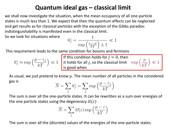
Quantum ideal gas classical limit we shall now investigate the situation, when the mean occupancy of all one-particle states is much less than 1. We expect that then the quantum effects can be neglected and get results as for classical particles with the exception of the Gibbs paradox: indistinguishability is manifested even in the classical limit. So we look for situations where This requirement leads to the same condition for bosons and fermions If this condition holds for ? = 0, then it holds for all ?, so the classical limit is good when As usual, we just pretend to know ?. The mean number of all particles in the considered gas is The sum is over all the one-particle states. It can be rewritten as a sum over energies of the one particle states using the degeneracy ?(?) The sum is over all the (discrete) values of the energies of the one-particle states.

Quantum ideal gas classical limit The discrete summation can be approximate by integrating over almost continuous spectrum of energies as where ?(?) is our standard notation for the number of one-particle states with energies less than ?. For spinless particles we have (? is the mass of the particles ? = ?2/3). Let us note that the spin degeneracy survives the classical limit so for particles with spin we should include also the spin degeneracy factor ? (2 for the spin 1/2, 3 for the spin 1 etc.). The integration is trivial, we get where we have denoted The index Q in the notation suggests quantum volume . ??is the volume corresponding to the de Broglie s wavelength of a particle having the energy by the order of magnitude equal to ??. It is roughly a minimum volume required so that the particle can have such energy. Restricting to a smaller volume would lead (by uncertainty principle) to larger energy.

Quantum ideal gas classical limit The relation we more often use in the inverse form: to calculate ? when we know ?: We have calculated the chemical potential! Of course, the result is valid only in the classical limit, what requires or Intuitively we understand why this is the condition of classicality. ???is the minimal volume required by quantum mechanics for the gas so that its temperature (roughly kinetic energy per molecule) can be ?. If the available total volume is much larger than that, the de Broglie s waves are not squeezed by the gas container and particles behave as classical. Of course, this is a hand-waving argument, but perhaps there is a piece of truth in it.

Ideal gas classical limit grand partition function We shall demonstrate now the calculation of the grand partition function for an ideal gas in the classical limit. The gas microstate is given by the list of the occupational numbers, which we shall denote as The grand partition function is the sum over all gas microstates (over all possible lists}: Be careful and understand well what the symbols mean! The overall sum is over all possible infinite lists of occupational numbers. The sums in the exponent are over the occupational numbers in one specific list. Now exponent of a sum is a product of exponents: Now the most difficult (for understanding) rearrangement according to the distributive law. Symbolically but imprecisely: sum of products is the product of sums . Observe the difference: in the original expression the sum is over lists of numbers, in the transformed expression the sum is over all possible occupational number values for the specific state ?. So for fermions it is the sum of just two numbers 0, 1. You can understand that this is correct by inspecting small specific examples for the distributive law. Try hard, finally you will understand the distributive law!

Ideal gas classical limit grand partition function So far, our calculations were exact. Now we will do approximations of the classical limit. Firstly, in the classical limit there is no difference between bosons and fermions because the mean occupational numbers are very low. So we continue the calculations with fermions, where the sums are only over ??= 0,1. The classical limit also means so we approximate the logarithms We got just the sum over mean occupational numbers, what gives the total number of particles. So in the classical limit We have calculated the grand partition function! We were able to do it because of the classical limit but also because in the grand statistical sum there is no restriction for the one- particle states we sum over. For the canonical sum the restriction ??= ? would make a similar calculation more difficult. (Later we shall see that in classical (non-quantum) statistics the calculation of the canonical sum for ideal gas is easy!)

Ideal gas classical limit entropy Summarizing the results we have obtained we continue by calculating the entropy of an ideal gas in the classical limit. We start with the relation After substitution for ? and we get This formula is called Sackur-Tetrode equation for the entropy of monoatomic classical ideal gas. It demonstrates that the statistical physics is able to calculate the entropy absolutely: there is no arbitrary additive constants, while the phenomenological thermodynamics is able to determine entropy only up to an additive constant.

Fermi ideal gas at low temperatures Fermi-Dirac distribution in the limit ? 0 gives At ? = 0 all one-particle states below ? = ? are occupied, all states above ? are empty. So at ? = 0 chemical potential ? is equal to the energy of the highest occupied one-particle state. This energy is called the Fermi energy ??. The Fermi energy can easily be calculated if we realize that the number of one-particle states below ??must be equal to the total number of particles. (Do not forget ? = 2 for spin 1/2 particles.)

Fermi ideal gas at low temperatures or temperatures slightly above ? = 0 the chemical potential will be slightly higher then ??so the occupation numbers will be only slightly different from their values at ? = 0 for ? around ??in the interval with a width ??. (Red curve.) This qualitative picture will not change until the temperature reaches Fermi temperature ? ??= ??/?. Fermi gas below the Fermi temperature is called degenerate Fermi gas. As an example of degenerate fermi gas we can consider conduction electrons in metal. Of course, the electron gas is not ideal, the electron feel each other. We use this example only to demonstrate some features qualitatively. For metal potassium the electron density in the lattice is 1.34 1022cm 3and for the Fermi temperature we get ?? 24000 K.

Fermi ideal gas at low temperatures We shall calculate the degenerate fermion gas heat capacity work in the approximation ? = ??. We have intelligently written zero as this trick enables us to use the substitution For temperatures much lower than ??Fermi-Dirac function is constant (either 1 or 0) almost everywhere except around ??. So the derivative of the Fermi-Dirac function is nonzero only around ??.Therefore the slowly varying function ? (?) can be replaced by the constant value ? (??) and we get For ? ??we can replace the lower bound by

Fermi ideal gas at low temperatures The obtained result shows that the heat capacity of the conduction electron gas is negligible for ? ??. This is how quantum mechanics (which was not yet known) saved the statistical physics from being thrown away. The heat capacity of electrons (which were not yet known) did not influenced the heat capacity of the metal as given by the lattice of atoms and everything was ok with the predictions of statistical physics at normal temperatures.

Bose condensation Bosons are particles which can have any occupation numbers of the one-particle states. It means that at very low temperatures practically all bosons of an ideal bose gas can occupy the lowest-energy one particle state. It is, however, not a priori clear whether at low but finite temperatures like 1K still a majority of particles would occupy the lowest-energy one-particle state. We shall estimate what happens for liquid helium which we shall very roughly consider to be an ideal gas in a box 1 cm3containing 1022particles. The energy of the lowest one-particle states will be ?0= 10 18eV, the first higher state will have energy twice that big ?1= 2?0. The mean occupation number of the lowest state is Let us assume that a significant number of particles 1022is in the lowest state, then

Bose condensation Let us calculate for this value of ? the occupancy of the first higher state at ? = 1K. So really even at 1K almost all particles can be in the lowest one-particle state. This effect is called Bose condensation.

Bose condensation If low-state occupation numbers are very high, we cannot approximate various summations by integration like this A more appropriate approximation would be to include the contribution by the lowest state explicitly (in a discrete way, the lowest state does not contribute to the integral) as We have seen in our numerical estimates that for low temperatures both ?0and ? are approximately zero, so we can write The integral gives the number of particles in higher one-particle states ??. After suitable substitution we get for it

Bose condensation The integral can be calculated numerically and we get The Bose condensation will disappear for temperatures for which already practically all the particles are in higher states: ?? ?. So the Bose condensation is present (very roughly) for temperatures lower than