Introduction to Sampling Weights and Probability

 undefined
Introduction to weighting
February 28, 2020
Nadi, FIJI


Sampling
In the simplest case….
…we select n units from a population of N units.
From this sample, we want to produce estimates that are
representative of the whole population
, i.e. all N units.
But how do we do that when we only have
information for the n units in the sample?
Sampling weights
Sampling weights
or
weights
are:
•
used to ensure estimates produced from a sample are
representative of the target population
•
positive values
used to “rate-up” or adjust
the data collected
for each sample unit
•
calculated for and assigned to
each unit in the sample
•
adjustments for different probabilities of selection
between
units in a sample, either due to the sample design or
happenstance (e.g. non-response).
Sampling Weights
Sampling Weights - Selection
A typical weight for each household found in a household survey
may be composed as follows:
with
sel
representing
selection
,
ps
representing post -
stratification, and
nr
representing non-response.
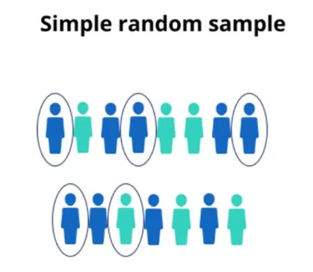
Probability of selection – SRS
Example: Probability of selection – SRS
Probability of selection – Stratified SRS
Example: Probability of selection –
Stratified SRS
Probability of selection – Two-stage selection
Probability of selection – 1
st
stage
Example: Probability of selection – Two-
stage selection
Probability of selection – 2
nd
stage
Probability of selection – Two-stage selection
Selection weight – Two-stage selection
Sampling Weights – Non-response
A typical weight for each household found in a household survey
may be composed as follows:
with
sel
representing selection,
ps
representing post -
stratification, and
nr
representing
non-response.
Non-Response
•
Nearly every survey has some degree of non-response for
which we can
make adjustments in the weights.
•
It is important to note that this is a non-response adjustment,
not a “correction.”
Without perfect information on all
variables, it is not possible to completely correct for non-
response.
•
The best we can do is
try to estimate the bias and make the
best adjustment possible
based on the information
available.
Non-Response (2)
Simplest form:
If your cluster has 12 households, but one
refuses, a simple calculation for the
nr
component of the
weights would be
=> Each remaining household counts a bit more than 1 to
make up for its missing neighbour.
=
> Selection weight for each household in the cluster is
adjusted upwards
(by 9%)
Weighting class
: divides the data into cells (such as age x
gender x geography) and assigns a correction factor based on
the cell response.
Sampling Weights – Post-stratification
A typical weight for each household found in a household survey
may be composed as follows:
with
sel
representing selection,
ps
representing
post -
stratification,
and
nr
representing non-response.
Post-Stratification
Post stratification is generally the last step in the process and
adjusts weighted totals to known population totals and has
been shown in the literature to reduce overall variance.
Example:
Selection weight for each person in
Maryland
is
adjusted
upwards
(by approx. 9%)
Selection weights for each person in
Virgina and DC
are
adjusted downwards
(by approx. 7% and 10% respectively)
Reasons for Weighting
Kish (1992) identifies
six reasons for weight
ing survey data prior
to analysis:
1.
To reflect
differential probabilities of selection
(=> produce
unbiased sample estimates)
2.
To
reduce biases introduced by errors in the sampling frame
3.
To
reduce bias introduced by non-response
4.
To
reduce sampling variance
, by making use of auxiliary
information (post-stratification)
5.
To produce
standardised, consistent estimates
6.
To produce approximately unbiased estimates from a sample
formed by combining other samples
Final Thoughts
Extra slides
Trimming
Trimming weights replaces outlier weights to reduce the
variance of the resulting estimations.
This causes some bias in the estimates and needs to be
carefully considered against gains in precision.
Trimming (2)
Trimming the outlier weights decreases the standard errors but
biases the estimate.
Sampling weights play a crucial role in producing estimates representative of the entire population from a sample. By assigning weights to sample units, adjustments are made to account for different probabilities of selection. Probability of selection, known as the sampling fraction, ensures fairness in representation. Learn about sampling weights, selection probabilities, and how they impact survey findings.

Download Presentation

Please find below an Image/Link to download the presentation.
The content on the website is provided AS IS for your information and personal use only. It may not be sold, licensed, or shared on other websites without obtaining consent from the author.If you encounter any issues during the download, it is possible that the publisher has removed the file from their server.
You are allowed to download the files provided on this website for personal or commercial use, subject to the condition that they are used lawfully. All files are the property of their respective owners.
The content on the website is provided AS IS for your information and personal use only. It may not be sold, licensed, or shared on other websites without obtaining consent from the author.
E N D
Presentation Transcript
Introduction to weighting February 28, 2020 Nadi, FIJI
Sampling In the simplest case . we select n units from a population of N units. From this sample, we want to produce estimates that are representative of the whole population, i.e. all N units. But how do we do that when we only have information for the n units in the sample?
Sampling weights Sampling weights or weights are: used to ensure estimates produced from a sample are representative of the target population positive values used to rate-up or adjust the data collected for each sample unit calculated for and assigned to each unit in the sample adjustments for different probabilities of selection between units in a sample, either due to the sample design or happenstance (e.g. non-response).
Sampling Weights A typical weight for each household found in a household survey may be composed as follows: ??????= ???? ??? ??? with sel representing selection, ps representing post - stratification, and nr representing non-response. ????= Selection weight or weight = Inverse of probability of selection
Sampling Weights - Selection A typical weight for each household found in a household survey may be composed as follows: ??????= ???? ??? ??? with sel representing selection, ps representing post - stratification, and nr representing non-response.
Probability of selection SRS Probability of selection for each household: ? =n N where: n = Number of households selected in the sample Nh = Number of households in the population Other terms for probability of selection selection probability, sampling fraction (f), inclusion probability, chance of selection Note that in SRS, every unit in the sample has the same sampling weight i.e. sampling weights are equal.
Example: Probability of selection SRS Consider an SRS of n = 200 households, from a population of N = 2,000 households. Probability of selection for each household: ? =n n N N = 2,000 = 200 2,000 = 200 = 1 1 1 10 0 = 0.1 or 10% = 0.1 or 10% Selection weight for each household in stratum h = inverse of the probability of selection: sel h h=1 1 P P=N N n n=2,000 2,000 200 w wsel 200= 10 = 10
Probability of selection Stratified SRS Probability of selection for each household in strata h: ?h=nh where: nh= Number of households selected in strata h Nh= Number of households (population) in strata h Nh Note that in more complex designs (stratified, two-stage), the sampling weights can vary between units or households unlike SRS, every unit in the sample has the same sampling weight.
Example: Probability of selection Stratified SRS Probability of selection and weight for each household in strata h: ?h h=n nh h sel h h=1 1 P Ph h=N Nh h and w wsel N Nh h n nh h Population (Nh) Sample size (nh) Probability of selection (Ph) =200/2,000 =0.1 or 10% =200/1,000 =0.2 or 20% Selection weight (w sel) Province 1 2,000 200 =2,000/200 = 10 =1,000/200 = 5 Province 2 1,000 200
Probability of selection Two-stage selection If there are 2 stages to sample selection then there are 2 stages in calculating the probability of selection for each household: 1. the probability of selecting 1 PSU (EA) i within stratum h = ?hi 2. the probability of selecting 1 household j within the selected PSU (EA) i =?ij The probability of selecting 1 household j in PSU (EA) i in stratum h, is the product of these 2 probabilities, i.e. ?hij= ?hi x?ji
Probability of selection 1st stage Probability of selecting 1 PSU (EA) i, within stratum h: ?hi= ?h Ni where: Probability Proportional to Size (PPS) sampling has been used to select PSUs within each EA and kh= Number of PSUs (EAs) selected in strata h Ni= Number of households in PSU i (e.g. from previous Census) Nh= Number of households in stratum h (e.g. from previous Census) Nh
Example: Probability of selection Two- stage selection Probability of selecting PSU (EA) i, within stratum h: ?hi= ?h Ni Nh If: stratum h contains Nh= 2,000 households (based on previous Census) we select ?h=10 PSUs from stratum h using PPS sampling, and PSU i containsNi= 70 households (based on previous Census) Then the probability of selecting PSU (EA) i within stratum h under PPS sampling is: ?hi= ?h Ni Nh =?? 70 70 2,000 2,000 = 0.35 = 0.35
Probability of selection 2nd stage Probability of selecting household j, within PSU (EA) i: nj Ni ?ij= where: nj= Number of households interviewed in PSU i (i.e. achieved cluster size in PSU i) Ni*= Number of households in PSU i (e.g. from Household listing)
Probability of selection Two-stage selection The probability of selecting household j in PSU (EA) i in stratum h, is the product of these 2 probabilities, i.e. ?hij = ?hi x ?ij= ?h Ni nj Ni Nh x where Probability Proportional to Size (PPS) sampling has been used to select PSUs within each EA, and: kh= # of PSUs (EAs) selected in strata h Ni = # of households in PSU i (e.g. from previous Census) Nh= # of households in stratum h (e.g. from previous Census) nj= # of households interviewed in PSU i Ni* = # of households in PSU i (e.g. from Household listing)
Selection weight Two-stage selection The probability of selecting household j in PSU (EA) i in stratum h is: ?hij = ?hi x ?ij= ?h Ni nj Ni Nh x So: the selection weight for household j in PSU (EA) i in stratum h is: ????= selection weight for household j in PSU (EA) i in stratum h = inverse of probability of selection = 1 1 ?h hij ij
Sampling Weights Non-response A typical weight for each household found in a household survey may be composed as follows: ??????= ???? ??? ??? with sel representing selection, ps representing post - stratification, and nr representing non-response.
Non-Response Nearly every survey has some degree of non-response for which we can make adjustments in the weights. It is important to note that this is a non-response adjustment, not a correction. Without perfect information on all variables, it is not possible to completely correct for non- response. The best we can do is try to estimate the bias and make the best adjustment possible based on the information available.
Non-Response (2) Simplest form: If your cluster has 12 households, but one refuses, a simple calculation for the nr component of the weights would be 11 12 1 12 11= 1.09 = => Each remaining household counts a bit more than 1 to make up for its missing neighbour. => Selection weight for each household in the cluster is adjusted upwards (by 9%) Weighting class: divides the data into cells (such as age x gender x geography) and assigns a correction factor based on the cell response.
Sampling Weights Post-stratification A typical weight for each household found in a household survey may be composed as follows: ??????= ???? ??? ??? with sel representing selection, ps representing post - stratification, and nr representing non-response.
Post-Stratification Post stratification is generally the last step in the process and adjusts weighted totals to known population totals and has been shown in the literature to reduce overall variance. Example: Weighted Total Population from Survey Maryland 5,245,757 Virginia 8,475,901 DC 662,842 Known Population 5,699,478 7,882,590 599,657 Adjustment Factor* 1.0865 0.9300 0.9047 State *Adjustment factor = ??? Selection weight for each person in Maryland is adjusted upwards (by approx. 9%) Selection weights for each person in Virgina and DC are adjusted downwards (by approx. 7% and 10% respectively)
Reasons for Weighting Kish (1992) identifies six reasons for weighting survey data prior to analysis: 1. To reflect differential probabilities of selection (=> produce unbiased sample estimates) 2. To reduce biases introduced by errors in the sampling frame 3. To reduce bias introduced by non-response 4. To reduce sampling variance, by making use of auxiliary information (post-stratification) 5. To produce standardised, consistent estimates 6. To produce approximately unbiased estimates from a sample formed by combining other samples
Final Thoughts Coming back to the formula: w = w w w final sel ps nr The factors represent the importance given to different sources of evidence. ???? is calculated by us through our direct actions. We can be very confident of the quality of this calculation. ??? is based on an external source. We have to decide how confident we are in the reliability of that source. ??? is based on theory. Since there is no way to empirically prove the theory our level of confidence is based on the literature - and how closely we feel that our situation matches this literature.
Trimming Trimming weights replaces outlier weights to reduce the variance of the resulting estimations. This causes some bias in the estimates and needs to be carefully considered against gains in precision. Distribution of Un-Trimmed Sampling Weights .002 .0015 Density .001 5.0e-04 0 0.00 1000.00 2000.00 3000.00 4000.00 Household weighting coefficient Source: KHBS 2004/2005
Trimming (2) Trimming the outlier weights decreases the standard errors but biases the estimate. Mean 6.899 6.882 6.875 6.895 6.964 Std. Err. 0.434 0.429 0.421 0.422 0.386 CV untrimmed 99 95 90 75 0.878 0.830 0.760 0.713 0.544


")


")