Hash Tables

Hash Tables
Comp 550

Dictionary
•
Dictionary:
–
Dynamic-set data structure for
storing items indexed using
keys
.
–
Supports
operations: Insert, Search, and Delete
(
take
O
(1) time
)
.
–
Applications:
•
Symbol-table of a compiler.
•
Routing tables for network communication.
•
Associative arrays (python)
•
Page tables, spell checkers, document fingerprints, …
•
Hash Tables:
–
Effective implementations of dictionaries.
Comp 550
Dictionary by Direct-address Tables
•
Direct-address Tables are
ordinary arrays
.
•
Support direct addressing by key values
.
–
Element whose key is
k
is obtained by indexing into
the
k
th
position of the array.
•
Applicable
when we can afford to allocate an
array with one position for every possible key.
–
i.e.
when the universe of keys
U
is small
.
•
Dictionary operations
(search, insert, delete) can
be implemented to each take
O
(1) time
.
–
Straightforward details in CLRS 11.1.
Comp 550
Hashing
0
m
–1
h
(
k
1
)
h
(
k
4
)
h
(
k
2
)
h
(
k
3
)
U
(
universe of keys)
K
(actual
keys)
k
1
k
2
k
3
k
5
k
4
h
(
k
2
)
Comp 550
n
=
|
K
|
<< |
U
|.
key
k
“hashes”
to slot
T
[
h
[
k
]]
hash table
T
[0
..m
–1]
.
h
:
U
{0,
1
,…, m
–1}
Dictionary by Hash Tables
•
Notation:
–
U
– Universe of all possible keys.
–
K
– Set of keys actually stored in the dictionary.
–
n
=
|
K
|
<< |
U
|.
•
Hash tables
use arrays of
size
m
=
(
n
):
–
Define functions that map keys to slots of the hash table.
–
Resolve collisions, since many keys map to same slot.
–
Support search, insert, delete, but not always O(1) worst-case.
•
Hash function
h
:
U
{0,
1
,…, m
–1}
maps keys
from
U
to
the slots of a hash table
T
[0
..m
–1]
.
–
key
k
maps or
“hashes”
to slot
T
[
h
[
k
]].
Comp 550
Hashing
0
m
–1
h
(
k
1
)
h
(
k
4
)
h
(
k
2
)
h
(
k
3
)
U
(
universe of keys)
K
(actual
keys)
k
1
k
2
k
3
k
5
k
4
collision
h
(
k
2
)=
h
(
k
5
)
Comp 550
Two questions:
•
1. How can we choose the hash function to
minimize collisions?
•
2. What do we do about collisions when they
occur?
Comp 550
Hash table design considerations
•
Collision resolution
–
separate chaining CLRS 11.2
•
Hash function design
–
Minimize collisions by spreading keys evenly
–
Collisions must occur because we map many-to-one
•
Collision resolution
–
open address CLRS 11.4
–
perfect hashing CLRS 11.5
•
Worst- and average-case times of operations
Comp 550
Collision Resolution by Chaining
0
m
–1
h
(
k
1
)=
h
(
k
4
)
h
(
k
2
)=
h
(
k
5
)=
h
(
k
6
)
h
(
k
3
)=
h
(
k
7
)
U
(
universe of keys)
K
(actual
keys)
k
1
k
2
k
3
k
5
k
4
k
6
k
7
k
8
h
(
k
8
)
X
X
X
Comp 550
k
5
Collision Resolution by Chaining
0
m
–1
U
(
universe of keys)
K
(actual
keys)
k
1
k
2
k
3
k
5
k
4
k
6
k
7
k
8
k
4
k
1
k
6
k
2
k
7
k
3
k
8
Comp 550
Hashing with Chaining
Dictionary Operations:
•
Chained-Hash-Insert (
T, x
)
–
Insert
x
at the head of list
T
[
h
(
key
[
x
])].
–
Worst-case complexity:
O
(1).
•
Chained-Hash-Search (
T, k
)
–
Search an element with key
k
in list
T
[
h
(
k
)].
–
Worst-case complexity: proportional to length of list.
•
Chained-Hash-Delete (
T, x
)
–
Delete
x
from the list
T
[
h
(
key
[
x
])].
–
Worst-case complexity: search time +
O
(1).
•
Need pointer to preceding element, or a doubly-linked list.
Comp 550
Analysis of Chained-Hash-Search
Worst-case search time:
time to compute
h
(
k
) +
(
n
).
Average time:
depends on how
h
distributes keys among slots.
•
Assume
–
Simple uniform hashing
.
•
Any key is equally likely to hash into any of the slots,
independent of where any other key hashes to.
–
O
(1) time to compute
h
(
k
)
.
•
Define
Load factor
=
n
/
m
= average # of keys per slot.
–
n
– number of keys stored in the hash table.
–
m
– number of slots = # linked lists
.
Comp 550
Some results
Comp 550
Theorem:
An unsuccessful search takes expected time
Θ
(1+
α
).
Theorem:
A successful search takes expected time
Θ
(1+
α
).
Theorem:
For the special case with
m=n
slots
,
with probability
at least 1-1/
n,
the longest list is
O(ln
n /
ln ln
n
).
Expected Cost of an Unsuccessful Search
Assume:
Any key not already in the table is equally likely to
hash to any of the
m
slots.
Proof:
•
We must follow pointers to end of list
T
[
h
(
k
)], which has
α
items,
so we expect 1+
α
pointer accesses.
•
Adding the time to compute the hash function, expected
total time remains
Θ
(1+
α
).
Key fact:
average bin size is
α
=
n/m.
Theorem:
An unsuccessful search takes expected time
Θ
(1+
α
).
Comp 550
Expected Cost of a Successful Search
Note:
Despite the similar look, this is very different from the previous
– i.e., we never look at the empty bins, but often at full ones!
Assume:
the element being searched for is equally likely to be any of
the
n
elements in the table.
Proof:
•
To find
x
we look first at all elements inserted
after
x
, then at
x.
(Think of inserting in reverse order -- becomes 1+the number already in bucket!)
•
Let
X
ij
=
IV{keys i
&
j
hash to same slot} Pr(
X
ij
=
1) = 1/
m
by s.u.h.
•
We want
•
So, we expect 1+
α
/2 pointer accesses.
Theorem:
A successful search takes expected time
Θ
(1+
α
).
Comp 550
Bounding the Size of Longest List
Proof:
•
Let
Z
i,k
=
IRV{key i
hash to slot
k
} Pr(
Z
i,k
=
1) = 1/
m
by s.u.h.
•
The probability that a particular slot
k
receives >
κ
keys is (letting
m=n
)
•
If we choose
κ
= 3 ln
n /
ln ln
n
, then
κ
! >
n
2
and 1/
κ
! < 1/
n
2
.
•
Thus, the probability that any
n
slots receives >
κ
keys is < 1/
n
.
•
With probability at least 1-1/
n,
Theorem:
For the special case with
m=n
slots
,
with probability at least 1-1/
n,
the longest list is
O(ln
n /
ln ln
n
).
Comp 550
Size of Longest List with 2 Choices
Proof idea:
•
The height of a ball is
i
if it was the
i-
th ball to be placed in it's bin.
•
Note: (total # of balls of height
i
) ≥ (total # of bins with
≥ i
balls)
•
Let
i
be the fraction of bins with
≥
i
balls. Note
2
≤1/2.
•
Pr[ ball has height
≥ i
+ 1]
≤
i
2
,
since to place a ball at height
i+1
we must select 2 bins of height ≥
i
. So we expect
i+1
≤
i
2
.
•
•
We are unlikely to see more than
i
= O(lg lg
n
) balls in a bin.
Theorem:
Using
m=n
slots and 2 hash functions,
placing each item in the shorter of the two lists, then
with probability at least 1-1/
n,
the longest list is
O(lg lg
n
).
Comp 550
Implications for separate chaining
•
If
n
=
O
(
m
), then load factor
=
n
/
m
=
O
(
m
)/
m
=
O
(1).
Search takes constant time on average
.
•
Deletion takes
O
(1) worst-case time if you have a pointer
to the preceding element in the list.
•
Hence, for
hash tables with chaining,
all dictionary
operations take
O
(1) time on average
,
given the
assumptions of simple uniform hashing and O(1) time hash
function evaluation.
•
Extra memory (& coding) needed for linked list pointers.
•
Can we satisfy the simple uniform hashing assumption?
Comp 550
Good hash functions CLRS 11.2
Comp 550
Good Hash Functions
•
Recall the assumption of
simple uniform hashing
:
–
Any key is equally likely to hash into any of the slots,
independent of where any other key hashes to.
–
O
(1) time to compute
h
(
k
).
•
Hash values should be independent of any
patterns that might exist in the data
.
–
E.g. If each key is drawn independently from
U
according to a probability distribution
P
, we want
for all
j
[
0
…m–
1],
k
:
h
(
k
)
= j
P
(
k
)
= 1/m
•
Often
use heuristics
, based on the domain of the
keys, to create a hash function that performs
well.
Comp 550
Keys as Natural Numbers
•
Let’s assume that keys are natural numbers,
even if we have to encode them to make them
so.
•
Example:
Interpret a character string as an
integer expressed in some radix notation. E.g.
“CLRS”:
–
ASCII values: C=67, L=76, R=82, S=83.
–
Use base 2
7
=128 to cover all basic ASCII values.
–
So, CLRS = 67
·128
3
+76 ·128
2
+ 82·128
1
+ 83·128
0
= 141,764,947.
–
Why not just sum the ASCII values?
Comp 550
“Division Method” (mod
p
)
•
Map each key
k
into one of the
m
slots by taking the
remainder of
k
divided by
m
. That is,
h
(
k
)
= k
mod
m
•
Example:
m
= 31 and
k
= 78
h
(
k
) = 16.
•
Advantage:
Fast, since requires just one division
operation.
•
Disadvantage:
For some values, such as
m=2
p
, the
hash depends on just a subset of the bits of the key.
•
Good choice for
m
:
–
Primes are good, if not too close to power of 2 (or 10).
Comp 550
Multiplication Method
•
Map each key
k
to one of the
m
slots indicated by the
fractional part of
k
times a chosen real 0
< A <
1.
•
That is,
h
(
k
)
=
m
(
kA
mod
1)
=
m
(
kA
–
kA
)
•
Example:
m =
1000
, k =
123
, A
0.6180339887
…
h
(
k
)
=
1000(123
·
0.6180339887 mod
1)
=
1000
·
0.018169...
=
18.
•
Disadvantage:
A bit slower than the division method.
•
Advantage:
Value of
m
is not critical.
•
Details on next slide
Comp 550
Multiplication Mthd. – Implementation
Simple implementation for
m
a power of 2.
•
Choose
m
= 2
p
, for some integer
p
.
•
Let the word size of the machine be
w
bits.
Pick a
w
-bit 0 <
s
< 2
w
.
Knuth suggests
(
5 – 1)·2
w-1
.
•
Let
A
=
s
/2
w
. (We need 0<
A
<1.)
•
Assume that key
k
fits into a single word. (
k
takes
w
bits.)
•
Compute
k
s
=
r
1
·2
w
+
r
0
•
The integer part of
kA
=
r
1
, drop it.
•
Take the first
p
bits of
r
0
by
r
0
<<
p
Comp 550
Open Addressing
•
Idea:
–
Store all
n
keys in the
m
slots of the hash table itself.
What can you say about the load factor
=
n/m
?
–
Each slot contains either a key or NIL.
–
To
search
for key
k
:
•
Examine slot
h
(
k
). Examining a slot is known as a
probe
.
•
If slot
h
(
k
) contains key
k
, the search is successful. If the slot contains
NIL, the search is unsuccessful.
•
There’s a third possibility:
slot
h
(
k
) contains a key that is not
k
.
–
Compute the index of some other slot, based on
k
and which probe we are
on.
–
Keep probing until we either find key
k
or we find a slot holding NIL.
•
Advantages:
Avoids pointers; so less code, and we can
dedicate the memory to the table.
Comp 550
Open addressing
0
m
–1
h
(
k
1
)
h
(
k
4
)
h
(
k
2
)
h
(
k
3
)
U
(
universe of keys)
K
(actual
keys)
k
1
k
2
k
3
k
5
k
4
collision
h
(
k
2
)=
h
(
k
5
)
h
(
k
5
)+1
Comp 550
Probe Sequence
•
Sequence of slots examined during a key search
constitutes a
probe sequence
.
•
Probe sequence must be a permutation of the slot
numbers.
–
We examine every slot in the table, if we have to.
–
We don’t examine any slot more than once.
•
One way to think of it: extend hash function to:
–
h
:
U
{0, 1, …, m
– 1}
{0, 1, …, m
– 1}
probe number slot number
Comp 550
Universe of Keys
Operations: Search & Insert
•
Search
looks for key
k
•
Insert
first searches for a slot, then inserts (line 4).
Comp 550
Hash-Insert(
T
,
k
)
1.
i
0
2.
repeat
j
h
(
k, i
)
3.
if
T
[
j
] = NIL
4.
then
T
[
j
]
k
5.
return
j
6.
else
i
i +
1
7.
until
i = m
8.
error
“hash table overflow”
Deletion
•
Cannot just turn the slot containing the key we want to
delete to contain NIL.
Why?
•
Use a special value
DELETED
instead of NIL when marking
a slot as empty during deletion.
–
Search
should treat DELETED as though the slot holds a key that
does not match the one being searched for.
–
Insert
should treat DELETED as though the slot were empty, so
that it can be reused.
•
Disadvantage:
Search time is no longer dependent on
.
–
Hence, chaining is more common when keys have to be
deleted.
Comp 550
Computing Probe Sequences
•
The ideal situation is
uniform hashing
:
–
Generalization of simple uniform hashing.
–
Each key is equally likely to have any of the
m
! permutations of
0, 1,…,
m
–1
as its probe sequence.
–
It is
hard to implement
true uniform hashing.
•
Approximate
with techniques that guarantee to probe a
permutation of [0…
m
–1], even if they don’t produce all
m
! probe
sequences
–
Linear Probing.
–
Quadratic Probing.
–
Double Hashing.
Comp 550
Linear Probing
•
h
(
k
,
i
) = (
h
(
k,0
)+
i
) mod
m
.
•
The initial probe determines the entire probe sequence.
•
Suffers from
primary clustering
:
–
Long runs of occupied sequences build up.
–
Long runs tend to get longer, since an empty slot preceded by
i
full slots gets filled next with probability (
i
+1)/
m
.
Comp 550
key
Probe number
Original hash function
Quadratic Probing
•
h
(
k,i
)
=
(
h
(
k
)
+ c
1
i + c
2
i
2
)
mod
m
c
1
c
2
•
Can suffer from
secondary clustering
Open addressing with linear probing
0
m
–1
h
(
k
1
)
h
(
k
4
)
h
(
k
2
)
h
(
k
3
)
U
(
universe of keys)
K
(actual
keys)
k
1
k
2
k
3
k
5
k
4
collision
h
(
k
2
)=
h
(
k
5
)
h
(
k
5
)+1
Comp 550
Double Hashing
•
h
(
k,i
)
=
(
h
1
(
k
)
+ i h
2
(
k
))
mod
m
•
Two auxiliary hash functions
.
–
h
1
gives the initial probe.
h
2
gives the remaining probes.
•
Must have
h
2
(
k
) relatively prime to
m
, so that the probe
sequence is a full permutation of
0, 1,…,
m
–1
.
–
Choose
m
to be a power of 2 and have
h
2
(
k
) always return an
odd number. Or,
–
Let
m
be prime, and have 1 <
h
2
(
k
) <
m
.
•
(
m
2
) different probe sequences
.
–
One for each possible combination of
h
1
(
k
) and
h
2
(
k
).
–
Close to the ideal uniform hashing.
Comp 550
key
Probe number
Auxiliary hash functions
Open addressing with double hashing
0
h
1
(
k
1
)
h
1
(
k
4
)
h
1
(
k
2
)
h
1
(
k
3
)
U
(
universe of keys)
K
(actual
keys)
k
1
k
2
k
3
k
5
k
4
collision
h
1
(
k
2
)=
h
1
(
k
5
)
Comp 550
Analysis of Open-address Hashing
•
Analysis is in terms of load factor
=
n/m
.
•
Assumptions:
–
The table never completely fills, so
n
<
m
and
< 1
.
–
uniform hashing
(all probe sequences equally likely)
–
no
deletion
–
In a successful search, each key is equally likely to be
searched for.
Comp 550
Expected cost of an
successful
search
Proof:
Let
P
k
= IRV{the first k
–
1 probes hit occupied slots}
The expected number of probes is just
•
If
α
is a constant, search takes
O
(1) time.
•
Corollary:
Inserting an element into an open-address
table takes
≤
1/(1–
α
)
probes on average.
Comp 550
Expected cost of a successful search
Proof:
•
A successful search for a key
k
follows the same probe sequence as
when
k
was inserted. Suppose that
k
was the (
i
+1)st key inserted.
–
At that time,
α
was
i
/
m
.
–
By the previous corollary, the expected number of probes
inserting
k
was
at most 1/(1–
i
/
m
) =
m
/(
m
–
i
).
•
We need to average over
i=1..n,
the positions for key
k
.
Comp 550
Analysis of Linear Probing
[PPR07]
•
Pagh, Pagh, and Ruzic showed two things:
–
If pairs of keys hash to independent locations, but
triples do not, then you can have expected
(log
n
) search time for linear probing.
–
If 5-tuples hash to independent locations, then
you can guarantee expected O(1) search time for
linear probing.
Comp 550
Sketch of analysis for
m
=3
n
[PPR07]
Imagine a binary tree over the hash table
A
[1..
m
]
•
A node at height
i
expects (1/3)·2
i
items;
call it
dangerous
if it has ≥(2/3)·2
i
items.
•
If key
k
finds a run at
h
(
k
) of between 2
i
and 2
i+1
items,
then the ancestor of
h
(
k
) at height
i
–2 is dangerous
or has a dangerous sibling.
•
Now, we want the probability that a bin, of expected size
μ=2
i
–2
/3, actually contains 2μ elements.
–
Pairs give bounds of O(1/μ), which is not enough, since
Σ
k
2
k
·O(1/2
k-2
) = O(lg n).
–
Quadruples give O(1/μ
2
), and Σ
k
2
k
·O(1/2
2(k-2)
)
= Σ O(2
-k
) = O(1).
Comp 550
Universal Hashing
•
A malicious adversary who has learned the hash function
can choose keys that map to the same slot, giving worst-
case behavior.
•
Defeat the adversary using
Universal Hashing
–
Use a different
random hash function
each time.
–
Ensure that the random hash function is
independent of the
keys
that are actually going to be stored.
–
Ensure that the random hash function is
“good”
by carefully
designing a
class of functions
to choose from.
Comp 550
Universal Set of Hash Functions
•
A finite collection of hash functions
H,
that map a universe of keys
U
into
{0,
1
,…, m–
1},
is
“
universal”
if, for every pair of distinct keys
k,l
U
,
the number of
h
H
with
h
(
k
)
=h
(
l
) is ≤ |
H
|/
m.
•
Key idea: use number theory to pick a large set
H
where
choosing
h
H
at random makes Pr{h
(
k
)
=h
(
l
) } = 1/
m
.
(A random
h
can be expected to satisfy simple uniform hashing.)
–
With table size
m,
pick a prime
p
≥ the largest key.
Define a set of hash functions for
a,b
[0…
p
–1],
a
>0,
h
a,b
(
k
) = ( (
ak + b
) mod
p
) mod
m.
•
Related to linear conguential random number generators (CLRS 31)
Comp 550
Example Set of Universal Hash Fcns
With table size
m,
pick a prime
p
≥ the largest key.
Define a set of hash functions for
a,b
[0…
p
–1],
a
>0,
h
a,b
(
k
) = ( (
ak + b
) mod
p
) mod
m.
Claim:
H is a 2-universal family
.
Proof: Let's fix
r≠s
and calculate, for keys
x ≠ y
,
Pr([(
ax + b
) =
r
(mod p)] AND [(
ay+b
) =
s
(mod
p
)]). We must have
a(x
–
y) = (r
–
s)
mod
p
, which is uniquely determines
a
over the field
Z
p
+
, so
b
=
r
–
ax
(mod
p
).
Thus, this probability is 1/
p
(
p
–
1).
Now, the number of pairs
r≠s
with
r = s
(mod
m
) is
p
(
p
–
1)/
m,
so
Pr[(
ax+b
mod
p
) = (
ay+b
mod
p
) (mod n)] = 1/
m
.
QED
Comp 550
Chain-Hash-Search with
Universal Hashing
Theorem:
Using chaining and universal hashing on key
k
:
•
If
k
is
not
in the table T
, the
expected length
of the list that
k
hashes to is
.
•
If
k
is
in the table T
, the
expected length
of the list that
k
hashes to is
1+
.
Proof:
X
kl
= IRV{h
(
k
)=
h
(
l
)}
. E[
X
kl
] = Pr{h
(
k
)=
h
(
l
)}
1/
m
.
If key
, expected # of pointer refs. is
If key
k
T
, expected # of pointer refs. is
Comp 550
Perfect Hashing [FKS82]
U
(
universe of keys)
K
(actual
keys)
k
1
k
2
k
5
k
4
k
6
k
7
k
3
k
7
k
3
Comp 550
Two consequences of
•
Recall our analyses for search with chaining:
we let
X
ij
=
IRV{keys i
&
j
hash to same slot}
Consider
m = n
2
:
•
If the average # of collisions < ½, then more than
half the time we have no collisions!
•
Pick a random universal hash function and hash
into table with
m
=
n
2
. Repeat
until no collision.
Note: Thm. 11.9 in CLRS; uses Markov inequality in proof.
Comp 550
Two consequences of
Consider
m=n
:
•
We can show that (list sizes)
2
add up to O(
n
)
–
Let
Z
i,k
=
IRV{key i
hashes to slot
k
}
–
Let
X
ij
=
IRV{keys i
&
j
hash to same slot}
Note: Thm. 11.10 in CLRS.
Comp 550
Two consequences of
•
Let
Z
i,k
=
IRV{key i
hashes to slot
k
}
Let
X
ij
=
IRV{keys i
&
j
hash to same slot}
Comp 550
Perfect Hashing
•
If you know the
n
keys in advance,
makes a hash table with O(
n
) size,
and worst-case O(1) lookup time.
•
Just use two levels of hashing:
A table of size
n
, then tables of size
n
j
2
.
•
Dynamic versions have been created, but are usually
less practical than other hash methods.
Key idea:
exploit both ends of space/#collisions tradeoff.
Comp 550
Hash tables are essential data structures that support efficient operations like insertion, search, and deletion. They find applications in symbol tables of compilers, routing tables for network communication, and more. To minimize collisions, choosing the right hash function is crucial. When collisions occur, different methods like separate chaining and open addressing can be employed for resolution. Learn about hash function design, collision resolution strategies, and the complexities involved in hash table operations.

Download Presentation

Please find below an Image/Link to download the presentation.
The content on the website is provided AS IS for your information and personal use only. It may not be sold, licensed, or shared on other websites without obtaining consent from the author.If you encounter any issues during the download, it is possible that the publisher has removed the file from their server.
You are allowed to download the files provided on this website for personal or commercial use, subject to the condition that they are used lawfully. All files are the property of their respective owners.
The content on the website is provided AS IS for your information and personal use only. It may not be sold, licensed, or shared on other websites without obtaining consent from the author.
E N D
Presentation Transcript
Hash Tables Comp 550
Dictionary Dictionary: Dynamic-set data structure for storing items indexed using keys. Supports operations: Insert, Search, and Delete (take O(1) time). Applications: Symbol-table of a compiler. Routing tables for network communication. Associative arrays (python) Page tables, spell checkers, document fingerprints, Hash Tables: Effective implementations of dictionaries. Comp 550
Hashing hash table T[0..m 1]. 0 U (universe of keys) h(k1) h(k4) k1 K k4 (actual keys) k2 h(k2) h(k2) k5 k3 h(k3) h : U {0,1, , m 1} n = |K| << |U|. key k hashes to slot T[h[k]] m 1 Comp 550
Hashing 0 U (universe of keys) h(k1) h(k4) k1 K k4 (actual keys) k2 collision h(k2) h(k2)=h(k5) k5 k3 h(k3) m 1 Comp 550
Two questions: 1. How can we choose the hash function to minimize collisions? 2. What do we do about collisions when they occur? Comp 550
Hash table design considerations Collision resolution separate chaining CLRS 11.2 Hash function design Minimize collisions by spreading keys evenly Collisions must occur because we map many-to-one Collision resolution open address CLRS 11.4 perfect hashing CLRS 11.5 Worst- and average-case times of operations Comp 550
Collision Resolution by Chaining 0 U (universe of keys) h(k1)=h(k4) X k1 k4 K (actual keys) X k2 h(k2)=h(k5)=h(k6) k6 k5 k7 k8 k3 X h(k3)=h(k7) h(k8) m 1 Comp 550
Collision Resolution by Chaining 0 U (universe of keys) k4 k1 k1 k4 K (actual keys) k2 k6 k6 k5 k2 k5 k7 k8 k3 k7 k3 k8 m 1 Comp 550
Hashing with Chaining Dictionary Operations: Chained-Hash-Insert (T, x) Insert x at the head of list T[h(key[x])]. Worst-case complexity: O(1). Chained-Hash-Search (T, k) Search an element with key k in list T[h(k)]. Worst-case complexity: proportional to length of list. Chained-Hash-Delete (T, x) Delete x from the list T[h(key[x])]. Worst-case complexity: search time + O(1). Need pointer to preceding element, or a doubly-linked list. Comp 550
Analysis of Chained-Hash-Search Worst-case search time: time to compute h(k) + (n). Average time: depends on how h distributes keys among slots. Assume Simple uniform hashing. Any key is equally likely to hash into any of the slots, independent of where any other key hashes to. O(1) time to compute h(k). Define Load factor =n/m = average # of keys per slot. n number of keys stored in the hash table. m number of slots = # linked lists. Comp 550
Some results Theorem: An unsuccessful search takes expected time (1+ ). Theorem: A successful search takes expected time (1+ ). Theorem: For the special case with m=n slots, with probability at least 1-1/n, the longest list is O(ln n / ln ln n). Comp 550
Implications for separate chaining If n = O(m), then load factor =n/m = O(m)/m = O(1). Search takes constant time on average. Deletion takes O(1) worst-case time if you have a pointer to the preceding element in the list. Hence, for hash tables with chaining, all dictionary operations take O(1) time on average, given the assumptions of simple uniform hashing and O(1) time hash function evaluation. Extra memory (& coding) needed for linked list pointers. Can we satisfy the simple uniform hashing assumption? Comp 550
Good hash functions CLRS 11.2 Comp 550
Good Hash Functions Recall the assumption of simple uniform hashing: Any key is equally likely to hash into any of the slots, independent of where any other key hashes to. O(1) time to compute h(k). Hash values should be independent of any patterns that might exist in the data. E.g. If each key is drawn independently from U according to a probability distribution P, we want for all j [0 m 1], k:h(k) = j P(k) = 1/m Often use heuristics, based on the domain of the keys, to create a hash function that performs well. Comp 550
Division Method (mod p) Map each key k into one of the m slots by taking the remainder of k divided by m. That is, h(k) = k mod m Example: m = 31 and k = 78 h(k) = 16. Advantage: Fast, since requires just one division operation. Disadvantage: For some values, such as m=2p, the hash depends on just a subset of the bits of the key. Good choice for m: Primes are good, if not too close to power of 2 (or 10). Comp 550
Multiplication Method Map each key k to one of the m slots indicated by the fractional part of k times a chosen real 0 < A < 1. That is, h(k) = m (kA mod1) = m (kA kA ) Example: m = 1000, k = 123, A 0.6180339887 h(k) = 1000(123 0.6180339887 mod1) = 1000 0.018169... = 18. Disadvantage: A bit slower than the division method. Advantage: Value of m is not critical. Details on next slide Comp 550
Multiplication Mthd. Implementation Simple implementation for m a power of 2. Choose m = 2p, for some integer p. Let the word size of the machine be w bits. Pick a w-bit 0 < s < 2w. Knuth suggests ( 5 1) 2w-1. Let A = s/2w. (We need 0<A<1.) Assume that key k fits into a single word. (k takes w bits.) Compute k s = r1 2w+ r0 The integer part of kA = r1 , drop it. Take the first p bits of r0 by r0 << p w bits k s = A 2w binary point r1 r0 extract p bits h(k) Comp 550
Open Addressing Idea: Store all n keys in the m slots of the hash table itself. What can you say about the load factor = n/m? Each slot contains either a key or NIL. To searchfor key k: Examine slot h(k). Examining a slot is known as a probe. If slot h(k) contains key k, the search is successful. If the slot contains NIL, the search is unsuccessful. There s a third possibility: slot h(k) contains a key that is not k. Compute the index of some other slot, based on k and which probe we are on. Keep probing until we either find key k or we find a slot holding NIL. Advantages: Avoids pointers; so less code, and we can dedicate the memory to the table. Comp 550
Open addressing 0 U (universe of keys) h(k1) h(k4) k1 K k4 (actual keys) k2 collision h(k2) h(k2)=h(k5) h(k5)+1 k5 k3 h(k3) m 1 Comp 550
Probe Sequence Sequence of slots examined during a key search constitutes a probe sequence. Probe sequence must be a permutation of the slot numbers. We examine every slot in the table, if we have to. We don t examine any slot more than once. One way to think of it: extend hash function to: h : U {0, 1, , m 1} {0, 1, , m 1} probe number slot number Universe of Keys Comp 550
Operations: Search & Insert Hash-Insert(T, k) 1. i 0 2. repeatj h(k, i) 3. ifT[j] = NIL 4. thenT[j] k 5. return j 6. else i i + 1 7. until i = m 8. error hash table overflow Hash-Search (T, k) 1. i 0 2. repeat j h(k, i) 3. ifT[j] = k 4. thenreturn j 5. i i + 1 6. untilT[j] = NIL or i = m 7. return NIL Search looks for key k Insert first searches for a slot, then inserts (line 4). Comp 550
Deletion Cannot just turn the slot containing the key we want to delete to contain NIL. Why? Use a special value DELETED instead of NIL when marking a slot as empty during deletion. Search should treat DELETED as though the slot holds a key that does not match the one being searched for. Insert should treat DELETED as though the slot were empty, so that it can be reused. Disadvantage: Search time is no longer dependent on . Hence, chaining is more common when keys have to be deleted. Comp 550
Computing Probe Sequences The ideal situation is uniform hashing: Generalization of simple uniform hashing. Each key is equally likely to have any of the m! permutations of 0, 1, , m 1 as its probe sequence. It is hard to implement true uniform hashing. Approximate with techniques that guarantee to probe a permutation of [0 m 1], even if they don t produce all m! probe sequences Linear Probing. Quadratic Probing. Double Hashing. Comp 550
Linear Probing h(k, i) = (h(k,0)+i) mod m. key Probe number Original hash function The initial probe determines the entire probe sequence. Suffers from primary clustering: Long runs of occupied sequences build up. Long runs tend to get longer, since an empty slot preceded by i full slots gets filled next with probability (i+1)/m. Quadratic Probing h(k,i) = (h (k) + c1i + c2i2)mod m c1 c2 Can suffer from secondary clustering Comp 550
Open addressing with linear probing 0 U (universe of keys) h(k1) h(k4) k1 K k4 (actual keys) k2 collision h(k2) h(k2)=h(k5) h(k5)+1 k5 k3 h(k3) m 1 Comp 550
Double Hashing h(k,i) = (h1(k) + i h2(k))mod m key Probe number Auxiliary hash functions Two auxiliary hash functions. h1 gives the initial probe. h2 gives the remaining probes. Must have h2(k) relatively prime to m, so that the probe sequence is a full permutation of 0, 1, , m 1 . Choose m to be a power of 2 and have h2(k) always return an odd number. Or, Let m be prime, and have 1 < h2(k) < m. (m2) different probe sequences. One for each possible combination of h1(k) and h2(k). Close to the ideal uniform hashing. Comp 550
Open addressing with double hashing 0 U (universe of keys) h1(k1) =h1(k5)+ h2(k5) h1(k4) k1 K k4 (actual keys) k2 collision h1(k2) h1(k2)=h1 (k5) k5 k3 h1(k3) h1(k5)+ 2h2(k5) Comp 550
Analysis of Open-address Hashing Analysis is in terms of load factor = n/m. Assumptions: The table never completely fills, so n <m and < 1. uniform hashing (all probe sequences equally likely) no deletion In a successful search, each key is equally likely to be searched for. Comp 550
Expected cost of an successful search Theorem: Under the uniform hashing assumption, the expected number of probes in an unsuccessful search in an open-address hash table is at most 1/(1 ). Proof: Let Pk= IRV{the first k 1 probes hit occupied slots} The expected number of probes is just = 1 1 m k m k 1 1 k 0 m = 1 k k ( ) ( ) E P E P k k 1 k If is a constant, search takes O(1) time. Corollary: Inserting an element into an open-address table takes 1/(1 ) probes on average. Comp 550
Expected cost of a successful search Theorem: Under the uniform hashing assumption, the expected number of probes in a successful search in an open-address hash table is at most (1/ ) ln (1/(1 )). Proof: A successful search for a key k follows the same probe sequence as when k was inserted. Suppose that k was the (i+1)st key inserted. At that time, was i/m. By the previous corollary, the expected number of probes inserting k was at most 1/(1 i/m) = m/(m i). We need to average over i=1..n, the positions for key k. m i m n i i key for expected are probes 1 1 n n 1 1 1 1 1 m = = Thus, ( ) ln H H m m n 1 n m i = = 0 0 k Comp 550
Universal Hashing A malicious adversary who has learned the hash function can choose keys that map to the same slot, giving worst- case behavior. Defeat the adversary using Universal Hashing Use a different random hash function each time. Ensure that the random hash function is independent of the keys that are actually going to be stored. Ensure that the random hash function is good by carefully designing a class of functions to choose from. Comp 550
Universal Set of Hash Functions A finite collection of hash functions H, that map a universe of keys U into {0, 1, , m 1}, is universal if, for every pair of distinct keys k,l U, the number of h H with h(k)=h(l) is |H|/m. Key idea: use number theory to pick a large set H where choosing h H at random makes Pr{h(k)=h(l) } = 1/m. (A random h can be expected to satisfy simple uniform hashing.) With table size m, pick a prime p the largest key. Define a set of hash functions for a,b [0 p 1], a>0, ha,b(k) = ( (ak + b) mod p) mod m. Related to linear conguential random number generators (CLRS 31) Comp 550
Example Set of Universal Hash Fcns With table size m, pick a prime p the largest key. Define a set of hash functions for a,b [0 p 1], a>0, ha,b(k) = ( (ak + b) mod p) mod m. Claim: H is a 2-universal family. Proof: Let's fix r s and calculate, for keys x y, Pr([(ax + b) = r (mod p)] AND [(ay+b) = s (mod p)]). We must have a(x y) = (r s) mod p, which is uniquely determines a over the field Zp+, so b = r ax (mod p). Thus, this probability is 1/p(p 1). Now, the number of pairs r swith r = s (mod m) is p(p 1)/m, so Pr[(ax+b mod p) = (ay+b mod p) (mod n)] = 1/m. QED Comp 550
Chain-Hash-Search with Universal Hashing Theorem: Using chaining and universal hashing on key k: If k is not in the table T, the expected length of the list that k hashes to is . If k is in the table T, the expected length of the list that k hashes to is 1+ . Proof: Xkl = IRV{h(k)=h(l)}. E[Xkl] = Pr{h(k)=h(l)} 1/m. If key , expected # of pointer refs. is If key k T, expected # of pointer refs. is ( 1 + j i k T 1 ( ) 1 n n i = i = ( ) E X ij m m j j ) 1 m 1 m ( n n i = + = + + ) 1 1 1 E X ij 2 2 j Comp 550
Perfect Hashing [FKS82] k1 U (universe of keys) k4 k1 k4 k5 K (actual keys) k2 k6 k5 k7 k2 k3 k7 k6 k3 Comp 550
) 1 ( n n 2 = ( ) E X Two consequences of ij m i j Recall our analyses for search with chaining: we let Xij=IRV{keys i & j hash to same slot} Consider m = n2: If the average # of collisions < , then more than half the time we have no collisions! Pick a random universal hash function and hash into table with m=n2. Repeat until no collision. ( ) 1 2 1 n n i = ( ) E X ij 2 2 n j Note: Thm. 11.9 in CLRS; uses Markov inequality in proof. Comp 550
) 1 ( n n 2 = Two consequences of ( ) E X ij m i j Consider m=n: We can show that (list sizes)2 add up to O(n) Let Zi,k=IRV{key i hashes to slot k} Let Xij=IRV{keys i & j hash to same slot} ) ( ) ( 1 1 1 n i m k n i i + 2 ) = 2 ( ) ( E Z E X E n X , i k ii ij 1 j ) 1 m ( n n = + = 2 1 n n Note: Thm. 11.10 in CLRS. Comp 550
) 1 ( n n 2 = Two consequences of ( ) E X ij m i j Let Zi,k=IRV{key i hashes to slot k} Let Xij=IRV{keys i & j hash to same slot} ) ( 1 1 = ( ) = 2 ( ) ( )( ) E Z E Z Z n ) ) , , , i k i k j k 1 1 1 k m i n k m i n j ( ( E Z Z , , i k j k 1 , 1 i j n k ) m = = + ( ( 2 ) E X n E X X n ij ii ij 1 , 1 1 i j i n i j = + 2 ) ( ) ( E X E n X ii ij 1 1 i n i j ) 1 ( n n = + n m Comp 550
Perfect Hashing If you know the n keys in advance, makes a hash table with O(n) size, and worst-case O(1) lookup time. Just use two levels of hashing: A table of size n, then tables of size nj2. k1 k4 k5 k2 k6 k7 k3 Dynamic versions have been created, but are usually less practical than other hash methods. Key idea: exploit both ends of space/#collisions tradeoff. Comp 550


")


 1")
 1")
 1")