Getting Started with PlotLVP: Tips and Tricks

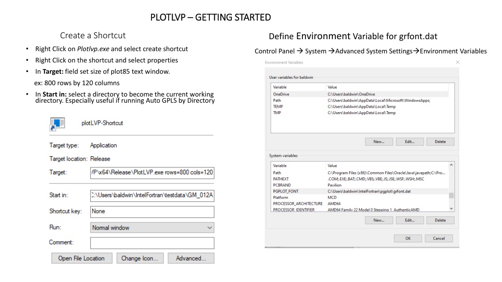
PLOTLVP PLOTLVP GETTING STARTED GETTING STARTED Create a Shortcut Define Environment Variable for grfont.dat Right Click on Plotlvp.exe and select create shortcut Control Panel System Advanced System Settings Environment Variables Right Click on the shortcut and select properties In Target: field set size of plot85 text window. ex: 800 rows by 120 columns In Start in: select a directory to become the current working directory. Especially useful if running Auto GPLS by Directory

NOTE: Only for PCs with an AMD processor. If you are using and Intel processor skip this step. At certain times while running PlotLVP you may encounter a popup window like this one. As stated this is just a warning message. However, if you close this window you will also terminate Plotlvp.exe. To prevent this situation from happening create the following environment variable. KMP_AFFINITY = disabled

Example Start in Start in folder Some useful files to have in the Start in folder: Template files for auto GPLS JCPDS files to display peak positions for known materials. A *.edf file - energy calibration file Note that there are subfolders in the Start in folder. These will be needed for Run Auto by Directory from the GPLS menu.

Notice that folder GM_A contains a template file and a med file. Folder GM_B contains only med files Folder GM_C contains med files and a template file

Some Basics Part I Read and plot a med file Menu: File Read File/Plot data Select a file with the navigation window.

Some Basics Part I continued Read and plot a JCPDS reference file Menu: JCPDS Read file/ Plot lines Select a file with the navigation window. Up to 5 reference files may be read/displayed. The Active Entry will be used for other procedures. See also JCPDS Profile/General Setup

Some Basics Part I continued Selecting a region of the plot window Bracket a region of the plot with two dots (periods) immediately followed by a third dot to expand the region. Red color added here for clarity. A slash (/) will expand that region and call GPLS. More on GPLS later. Left Right

Displaying Fluorescence Lines Fluorescence data for six elements are built in. Data for four more elements can be added on a rotating basis. The fifth element added will replace the first and so on. Select Add element . Here Hf and Y have been added, one at a time. Then Hf was selected.

Select Plot Lines

GPLS General Purpose Least Squares Step 1. Select the general refinement parameters 5 Cycles is generally sufficient. Set the number of peaks to fit. If the number of peaks will be different in different ranges you can select 0 and then use q for peak position after selecting the peaks. Not recommended when creating a template file. If a JCPDS reference file is active select peak position with the peak number from the reference file to tag hkl s. If fitting multiple peaks you can refine a single peak width or individual peak widths. Step 2. Read a data file. Step 3. Read and plot a JCPDS file. Not required but recommended to capture HKLs. Step 4. Optionally select multiple detectors from GPLS General Setup Step 5. Select a region of data with . . / Step 6. Follow the on screen directions. If you did step 3, remember to point to the peak with the appropriate number to capture the hkl indices. Note: If you want to sum the data from multiple detectors then select Sum detector-fast or Sum detector-slow. This needs to be done before reading the datafile. Fast just sums channel by channel. Slow sums by energy to match the energy from detector 1.

PlotLVP PlotLVP Plot window Hot Keys When the plot window is active: Pressing any key will display the character at the cursor position and print channel number, intensity, energy, d-spacing If a JCPDS reference material has been selected the number and shifted number keys point to the corresponding reference line. Information for that line can later be used by GPLS. E or e indicate the position corresponds to an energy peak and not a diffraction peak. The selection commands "..." and "../" will expand the range pointed to by the first two dots. A third dot will expand what is displayed, while the / will expand and invoke GPLS. N and n will read the next/previous data file in the sequence. Q or q will quit and return to the menu. S, s, esc: S and esc will redisplay the original data, and s will redisplay the current data selection. Position and JCPDS markers will be lost. Function keys F1 through F10 will select detectors 1-10 respectively. Calibration of each detector is maintained. With some keyboards, after pressing F10, you may have to press F1 before pressing any other function key. Control x, y and z will invoke the first, second and third template files respectively. "I" and "i" will increment/decrement the cell edges of the active JCPDS reference material , recalculate the d-spacing and replot the data. See menu item JCPDS Profile/General Setup to select the active JCPDS reference material. T or t decrement/increment edf parameter tth and replot. Must be activated. See E-caleb setup Y or y will reset the y-scale factor to that position P or p create a print file if a printer has been defined

Setting Up and Running Auto GPLS by Directory Prerequisites Read and plot a med file to initialize the graphics subsystem Create one or more template files and place in the appropriate directories. See previous slides. Read a JCPDS file optional. Will include HKL values in peak files. Tips and Hints Test settings with a few files first using hot keys N, n and control X If processing many files: Select suppress graphics in GPLS Auto Peakfit Setup Reduce Info messages to few or none in Utilities II menu. Be very careful if selecting Update template data

Flow Chart for Auto GPLS by Directory Flow Chart for Auto GPLS by Directory Current Working Directory More Subdirectories? 1. Program switches to the GPLS Working Directory Steps 1 and 2 2. A check is made for sub directories. No Yes 3. If there is a sub directory, switch to it. If no more sub directories go to step 8. Change Directory Is there a Template file? 4. Check for template file. Steps 3 and 4 5. If template file then use it. If no template file then continue using current template data. Yes No 6. Check for med or chi files. Read new Template data Finished Step 5 7. Process all the data files and return to step 2. More data files? Step 6 8. Finished! Yes Step 7 Process data

Setting Up and Running Auto GPLS by Directory with MED Files 1,2 1. 2. 3. 4. File type: MED (default) Working directory defaults to Start in directory (can be modified) Do not create individual pk files. Create Region and all.pks files. Checking Use Range 1 to control shift will have the template peak position replaced by the highest point if within 0.5 of range width of template peak position. Check Update Template data to shift all template data by shift of this peak. Range 1 must be a single peak. Do not Pause between regions or files and Skip confirmation of Template file. Not Creating template file, not Suppressing Graphics and not tweaking calibration Including Reject information in pks files and not linking to Celrf Reject peak if: Goodness of Fit exceeds 500, fit position moves by more than 7.5% of region width, or Intensity differs from template value by more than a factor of 8 or 5*Sig(I) > I (Note: fitted Intensity is area under curve and template is just one point.) If processing many files consider selecting Suppress Graphics and limiting output to text window (See Utilities II menu) 3 4 5 6 7 5. 6. 7. 8. 8 9.

Setting Up and Running Auto GPLS by Directory with CHI Files Select Fit2D/Chi Fit2D/Chi Chi Setup Chi Setup Check GPLS Chi Mode = 1 Set wavelength= 0.1847

Sample Directory Structure Sample Directory Structure Auto by Directory Auto by Directory with Chi files with Chi files Top level directory - The Working Directory D:\IntelFortran\testdata\ChiFiles\CaSiO3-DJW3 The Working Directory has two subdirectories AutoRun_111 AutoRun_211 Each subdirectory has a template file and Chi files

AutoGPLS setup - Chi files Set File Type to Chi Check the Working Directory Select other options as needed. Reduce the amount of printed output if desired Level 3 Few

Beginning and ending output Beginning and ending output - - Run Auto by Directory Run Auto by Directory Files created. Files created. Each subdirectory now has an all.pks A region.d1r1 and a ChiVsD.dat file.

More about the ChiVsD.dat File 1 Reflections : 72 datapoints HKL: 1 1 1 5. 2.0896 3. 1 10. 2.0713 770. 0 15. 2.0705 936. 0 20. 2.0699 875. 0 25. 2.0691 873. 0 30. 2.0680 880. 0 35. 2.0677 848. 0 40. 2.0673 943. 0 45. 2.0667 1048. 0 50. 2.0666 1193. 0 . . . 320. 2.0803 1010. 0 325. 2.0792 2120. 0 330. 2.0772 2913. 0 335. 2.0764 2845. 1 340. 2.0752 2224. 0 345. 2.0747 1457. 0 350. 2.0743 1121. 0 355. 2.0739 912. 0 360. 2.0734 678. 0 2.07569 0.00197 0.46831 Each data line contains Chi angle, d-spacing, Intensity and a rejection flag. Flag = 1 reject this point in any calculations. Last line contains: Linear fit: intercept, slope, correlation coefficient

Using the ChiVsD.dat File to get best fit Strain You can use the ChiVsD file to get a better estimate of the strain by optimizing the Chi zero value. Example 1. Read the ChiVsD file with default values in Chi Setup. Select Plot Strain function in Gpls General Setup

Strain plot confirms that the point with a d-space of 2.0896 should be rejected. Change the reject flag for this point in the ChiVsD.dat file to 1. The results almost the same as in the original ChiVsd.dat file. Notice that 2 of the 72 points were rejected.

The results somewhat improved. Slightly higher correlation coefficient. Notice that 3 of the 72 points were now rejected.

Using ChiVsD.dat Example 2 Apply a Chi Angle Offset of -35 degrees then increment by 5 degrees (Offset Inc) 15 times(# of incs) finding the best fit line. Results indicate that Chi zero is close to -30 degrees with a correlation coefficient 0.88.

Creating Template Files Template files provide the information necessary to fit peak data left and right backgrounds and peak position and intensity I. Manual Method. 1. Select Create template file in GPLS Auto Peakfit Setup 2. It is recommended that a JCPDS file be active to capture HKLs but this is not required. 3. Fit the desired peaks as described in Basics Part I. Do not select 0 peaks in GPLS General Setup. Use a discrete number of peaks. 4. When finished fitting peaks be sure to uncheck Create template file. II. Auto Generate from JCPDS 1. Select the menu item JCPDS Profile/General Setup 2. Peak Width is number of channels centered on Peak positions. Only reflections with Min intensity will be used. Select which JCPDS entry to use active entry. 3. Select the menu item JCPDS Create template file

Using Cell Refine Refining Unit Cell Parameters General Steps: 1. Read and plot a data file 2. Read and plot a JCPDS file 3. Create and read a template file. 4. Select Create pk files in GPLS -> Auto Peakfit Setup. Be sure Create Template file is not checked. 5. In Graphics window type Control X to invoke GPLS. A *.pk file should have been created. 6. Use Cell Refine-> Setup. Enter Cell parameters and refinement switches as appropriate. Example for Hexagonal System. Systematic Errors is not appropriate for energy dispersive data. Delta Q Reject is (Qc-Qo) (Q is 1/d2; Qo is Q observed, and Qc is Q calculated). 7. Use Cell Refine -> Refine. Select the pk file created in step 5. A listing file from the refinement will be created. 8. Alternatively, do steps 1-3, 6, and in step 4, Select Create pk files and Link to Celrf in GPLS -> Auto Peakfit Setup then step 5.

Data - - Quick Start: Quick Start: Processing Processing Ultrasonics Ultrasonics Data 1. Ultrasonics->Import Ultrasonics raw data 2. Ultrasonics->Read 3. Ultrasonics->Plot Waveform Must enter Q or q to enable next step Use n and N to read new files. 4. Ultrasonics->Select Segment 1 Point and hit any key to select the Left and then the Right side of segment 1. 5. Ultrasonics->Select Segment 2 Point and hit any key to select the Left side of segment 2. Segment 2 will have the same size as segment 1. 6. Ultrasonics->Plot Segments Use Hot Keys to overlap segments. Q or q when finished.

Data Hot Keys: Hot Keys: Processing Processing Ultrasonics Ultrasonics Data L l R r S s Q q + - [ ] < , > . D d U u / * ; ' n N Select left edge of zoomed region Select right edge of zoomed region Unzoom. Restore full pattern Quit graphics Scale segment 2 Up / Down Scale segment 1 Up / Down Shift segment 2 left Shift segment 2 right Shift segment 2 Down Shift segment 2 Up Divide / multiply horizontal shift amounts for segment 2 by 10 Divide / multiply vertical shift amounts for segment 2 by 10 Read next / previous file. Only active during 'Plot waveform'

Processing Processing Ultrasonics Ultrasonics Data Data Step by Step Part 1 Step by Step Part 1 Reading the data Reading the data On initial startup there are only two Ultrasonics options available: Import Ultrasonics raw data When selecteda navigation panel will open to allow you to pick a file. Once a file as been imported the Read option becomes available. Read: Prepares the imported data for ultrasonics processing. The Plot waveform option will then be available. See next slide. Get Scale/Shift Factors The default Scale factors for both segments are 5.0%. Horizontal and Vertical shifts are 0.5 and 0.02 respectively

ata Step by Step Part 2 Step by Step Part 2 Plotting the data Ultrasonics D Data Processing Processing Ultrasonics Plotting the data Plot waveform hotkeys Select left edge of zoomed region Select right edge of zoomed region Unzoom. Restore full pattern Read next / previous file. Quit graphics L l R r S s n N Q q You must enter Q or q to enable next step. Select Segment 1 The plot window can be either full screen or zoomed mode when you Quit graphics.

Data Step by Step Part 3 Step by Step Part 3 Selecting segments Processing Processing Ultrasonics Ultrasonics Data Selecting segments Select Segment 1 will replot the data. Point to the left edge of the segment and press any key. Then point to the right edge and press any key. The segment will be plotted. Select Segment 2 will now be available. Choosing it Will cause the full pattern to be plotted. Point to the left edge of segment 2 and press any key. The width of segment 2 will be the same as segment 1. Segment 2 is plotted and menu option Plot Segments is now available. Choosing this causes both segments to be plotted. The left segment is in black and the right is in red. Now ready to overlap segments.

Data Step by Step Part 4 Step by Step Part 4 - - Overlapping segments Processing Processing Ultrasonics Ultrasonics Data Overlapping segments Use these hot keys to overlay segment 2 onto segment1 + - Scale segment 2 Up / Down [ ] Scale segment 1 Up / Down < , Shift segment 2 left > . Shift segment 2 right D d Shift segment 2 Down U u Shift segment 2 Up / * Divide / multiply horizontal shift amount for segment 2 by 10 ; Divide / multiply vertical shift amount for segment 2 by 10 Q q Quit graphics when finished (Note: Data for illustration only. Not meant to represent good data.)

Processing Processing Ultrasonics Ultrasonics Data Data Hints and Hints and Tips Tips Inverting a waveform Inverting a waveform To invert a waveform: Set the corresponding segment s scale factor to negative 1. Select Ultrasonics Get Scale/Shift Factors 1. 2. Scale the segment Up or Down with the appropriate hot key: + - [ ]. Then shift accordingly. U or u(s) + or - 3. Reset the corresponding segment s scale factor back to a positive number.

Birch Murgnahan Equation of State The EoS parameters are initially taken from the active JCPDS entry and/or entered manually. One of two calculations can be made. 1. V0/V can be calculated if values for pressure and temperature are given. 2. Pressure can be calculated if volume and temperature are entered.

Birch Murgnahan Calculating V0/V Enter values for Temp and Pressure Click OK Values for Volume and V0/V have been calculated

Birch Murgnahan Calculating Pressure Pressure not yet calculated Select BM again and click OK Select BM. Enter values for Volume and Temp Click OK The pressure has now been calculated