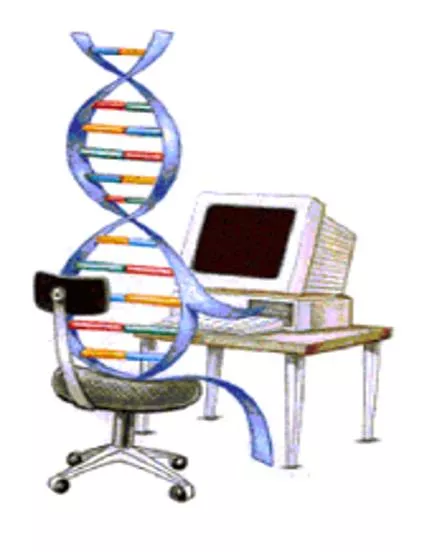
Genetic Algorithms and Natural Selection

 
Genetic Algorithms
 
2
 
 
3
 
History Of Genetic Algorithms
 
“Evolutionary Computing” was introduced in the 1960s by
I. Rechenberg
.
 
John Holland wrote the first book on Genetic Algorithms
Adaptation in Natural and Artificial Systems
 in 1975.
 
In 1992 
John Koza
 used genetic algorithm to evolve
programs to perform certain tasks. He called his method
Genetic Programming
”.
 
4
 
What Are Genetic Algorithms (GAs)?
 
 
   Genetic Algorithms are 
search
 and 
optimization
techniques based on Darwin’s Principle of 
Natural
Selection
.
 
5
 
 
Darwin’s Principle Of Natural Selection
 
IF there are organisms that reproduce, and
IF offsprings inherit traits from their progenitors, and
IF there is variability of traits, and
IF the environment cannot support all members of a
growing population,
THEN those members of the population with less-
adaptive traits (determined by the environment) will die
out, and
THEN those members with more-adaptive traits
(determined by the environment) will thrive
 
The result is the evolution of 
species
.
 
6
 
Basic Idea Of Principle Of Natural
Selection


“Select The Best, Discard The Rest”
 
7
 
An Example of Natural Selection
 
Giraffes have long necks
.
     
Giraffes with slightly longer necks could feed on leaves of higher
branches when all lower ones had been eaten off.
     
   They had a better chance of survival.
     
   Favorable characteristic propagated through generations of
giraffes.
     
   Now, evolved species has long necks.
 
     
NOTE:
 Longer necks may have been a deviant characteristic
(
mutation
) initially but since it was favorable, was propagated over
generations. Now an established trait.
 
     
So, some mutations are beneficial
.
 
8
 
Evolution Through Natural Selection
 
   Initial Population Of Animals
 
 
Struggle For Existence-Survival Of the Fittest
 
Surviving Individuals Reproduce, Propagate Favorable
Characteristics
 
 
Millions Of Years
 
Evolved Species
(Favorable Characteristic Now  A Trait Of Species)
 
9


Genetic Algorithms Implement
Optimization Strategies By Simulating
Evolution Of Species Through Natural
Selection.
 
Taxonomy
Search Techniques
Informed
Uninformed
BFS
DFS
A*
Hill Climbing
Simulated
Annealing
Evolutionary
Algorithms
Genetic
Programming
Genetic
Algorithms
Swarm
Intelligence
Evolutionary
Strategies
 
11
 
Working Mechanism Of GAs
Begin
Initialize
population
Optimum
Solution?
T=T+1
Selection
Crossover
Mutation
 
N
Evaluate Solutions
 
Y
Stop
 
T =0
 
12
 
Simple Genetic Algorithm
 
Simple_Genetic_Algorithm()
 
{
 
Initialize the Population;
 
Calculate Fitness Function;
 
While(Fitness Value != Optimal Value)
  
{
  
Selection
;
//Natural Selection, Survival Of Fittest
   
Crossover
;
//Reproduction, Propagate favorable characteristics
 
   
Mutation;
//Mutation
   
Calculate Fitness Function;
  
}
 
}
 
13
 
Nature to Computer Mapping
 
Components of a GA
 
A problem to solve, and ...
Encoding technique
  
(
gene, chromosome
)
Initialization procedure
  
(creation)
Evaluation function
  
(environment)
Selection of parents
  
(
reproduction)
Genetic operators
  
(mutation, recombination)
Parameter settings
  
(practice and art)
 
GA terminology
 
Population
The collection of potential solutions (i.e. all the chromosomes)
 
Parents/Children
Both are chromosomes
Children are generated from the parent chromosomes
 
Generations
Number of iterations/cycles through the GA process
 
16
 
Genotype, Phenotype, Population
 
Genotype
chromosome
Coding of chromosomes
coded string, set of coded strings
Phenotype
The physical expression
Properties of a set of solutions
Population – a set of solutions
deleted
members
parents
children
modified
children
evaluated children
chosen
parents
 
18
 
 
19
 
Encoding
 
   
The process of representing the solution in the form
of a 
string
 that conveys the necessary information.
 
Just as in a chromosome, each gene controls a particular
characteristic of the individual, similarly, each bit in the
string represents a characteristic of the solution.
 
20
 
Encoding Methods
 
Binary Encoding – 
Most common method of
encoding. Chromosomes are strings of 1
s and 0
s and each
position in the chromosome represents a particular
characteristic of the problem.


Genetic Algorithms:
Binary-Coded Representations
 
For Example, let’s say that we are trying to optimize the
following function,
f(x) = x
2
for 2 
 x 
 1
If we were to use binary-coded representations we would
first need to develop a mapping function form our genotype
representation (binary string) to our phenotype
representation (our C
andidate 
S
olution
). This can be done
using the following mapping function:
 
d(ub,lb,l,chrom) = (ub-lb) decode(chrom)/2
l
-1 + lb
 
Binary-Coded Representations
 
d(ub,lb,l,c) = (ub-lb) decode(c)/2
l
-1 + lb
 , where
ub
 
 
= 2,
lb
 
 
= 1,
l
 
  
= the length of the chromosome in bits
c
 
 
= the chromosome
The parameter, l, determines the accuracy (and resolution of
our search).
 
 
Binary Coded Representations
 
24
 
Encoding Methods (contd.)
 
Permutation Encoding –
 
Useful in ordering
problems such as the Traveling Salesman Problem (TSP).
Example. In TSP, every chromosome is a string of numbers,
each of which represents  a city to be visited.
 
25
 
Encoding Methods 
(contd.)
 
Value Encoding
 
Used in problems where
complicated values, such as real numbers, are used and
where binary encoding would not suffice.
    Good for some problems, but 
often necessary to develop
some specific crossover and mutation techniques for these
chromosomes.
 
Real-Coded Representations
 
27
 
Fitness Function


A fitness function quantifies the optimality of a
solution (chromosome) so that that particular
solution may be ranked against all the other
solutions.
 
A fitness value is assigned to each solution depending on
how close it actually is to solving the problem.
 
 Ideal fitness function correlates closely to goal + quickly
computable.
 
Example. In TSP, f(x) is sum of distances between the cities
in solution. The lesser the value, the fitter the solution is.
 
28
 
Recombination
 
   
The process that determines which solutions are to
be preserved and allowed to reproduce and which
ones deserve to die out.
 
The primary objective of the recombination operator is to
emphasize the good solutions
 and 
eliminate the bad
solutions
 in a population, 
while keeping the population
size constant.
 
“Selects The Best, Discards The Rest”.
 
“Recombination” is different from “Reproduction”.
 
29
 
Recombination
 
Identify the good solutions in a population.
 
Make multiple copies of the good solutions.
 
Eliminate bad solutions from the population so that
multiple copies of good solutions can be placed in
the population.
 
30
 
Roulette Wheel Selection
 
Each current string in the population has a slot assigned to
it which is in 
proportion to it’s fitness
.
 
We spin the weighted 
roulette wheel
 thus defined 
n 
times
(where 
n 
is the total number of solutions).
 
Each time Roulette Wheel stops, the string corresponding
to that slot is created.
 
    
Strings that are fitter are assigned a larger slot and hence
have a better chance of appearing in the new population.
 
Parent Selection Methods
 
31
 
Example Of Roulette Wheel Selection
 
32
 
Roulette Wheel For Example
 
Roulette wheel selection can be implemented as follows
1. 
Sum the fitnesses of all the population members. Call this
TF (total fitness).
   
Total=
1170
 
2. Generate a random number m, between 0 and TF.
   
m=300
3. Return the first population member whose fitness added to
the preceding population members is greater than or equal to
m.
  sum=169, sum=169+576 >m select second individual.
 
Pseudo code of Selection process
 
Function select(popsize, sumfitness, population) {
Begin
Partsum=0       j=0
rand= rand*sumfitness
Repeat
j=j+1
partsum=partsum+pop[j].fitness
Until(partsum>=rand) or (j=popsize)
Return individual number
Select=j
end
 
Tournament Selection
 
In Tournament Selection, q individuals are randomly
selected from the population and the best of the q
individuals is returned as a parent.
 
Selection Pressure increases as q is increased and
decreases a q is decreased.
 
Genetic Algorithms:
Genetic Procreation Operators
 
Genetic Algorithms typically use two types of operators:
Crossover (Sexual Recombination), and
Mutation (Asexual)
Crossover is usually the primary operator with mutation
serving only as a mechanism to introduce diversity in the
population.
However, when designing a GA to solve a problem it is
not uncommon that one will have to develop unique
crossover and mutation operators that take advantage of
the structure of the CSs comprising the search space.
 
37
 
Crossover
 
   
It is the process in which two chromosomes
(strings) combine their genetic material (bits) to
produce a  new offspring which possesses both their
characteristics.
 
Two strings are picked from the mating pool at random to
cross over.
 
The method chosen depends on the Encoding Method.
 
38
 
Crossover Methods
 
Single Point Crossover- 
A random point is chosen
on the individual chromosomes (strings) and the
genetic material is exchanged at this point.


39
 
Crossover Methods 
(contd.)
 
Single Point Crossover
 
40
 
Crossover  Methods 
(contd.)
 
Two-Point Crossover- 
Two random points are chosen
on the individual chromosomes (strings) and the genetic
material is exchanged at these points.


NOTE: These chromosomes are different from the last example.
 
41
 
Crossover Methods
 (contd.)
 
Uniform Crossover-
 
Each gene (bit) is selected
randomly from one of the corresponding genes of the
parent chromosomes.
 
NOTE: Uniform Crossover yields ONLY 1 offspring.
 
42
 
Crossover 
(contd.)
 
Crossover between 2 good solutions 
MAY NOT
ALWAYS
 yield a better or as good a solution.
 
Since parents are good, probability of the child
being good is high.
 
If offspring is not good (poor solution), it will be
removed in the next iteration during “Selection”.
 
Re
al-Coded Crossover Operators
 
For Real-Coded representations there exist a number of
other crossover operators:
Mid-Point Crossover,
Flat Crossover (BLX-0.0),
BLX-0.5
 
Mid-Point Crossover
 
Given two parents where X and Y represent a floating point
number:
Parent 1:    X
Parent 2:    Y
Offspring: (X+Y)/2
If a chromosome contains more than one gene, then this
operator can be applied to each gene with a probability of
P
mp
.
 
Flat Crossover (BLX-0.0)
 
Flat crossover was developed by Radcliffe (1991)
Given two parents where X and Y represent a floating point
number:
Parent 1:    X
Parent 2:    Y
Offspring: rnd(X,Y)
Of course, if a chromosome contains more than one gene
then this operator can be applied to each gene with a
probability of P
blx-0.0
.
 
BLX-
 
Developed by Eshelman & Schaffer (1992)
Given two parents where X and Y represent a floating point
number, and where X < Y:
Parent 1:    X
Parent 2:    Y
Let 
 = 
(Y-X), where 
 = 0.5
Offspring: rnd(X-
, Y+ 
)
Of course, if a chromosome contains more than one gene
then this operator can be applied to each gene with a
probability of P
blx-
.
 
Partially Matched Crossover (PMX)
PMX is similar to order-based crossover in that it can be
used for problems such as the travelling salesman problem.
An example is probably the best way to shows how PMX
operates. This example is taken from (Goldberg, 1989).
Given two parents, A and B, two crossover points are
chosen.
 
Now, looking at B, we consider the genes between the
crossover site. The first, 2, maps to 5 in parent A.
Therefore, we swap gene 2 with gene 5 in parent B.
Following the same principle we swap 3 and 6 and 10
and 7.
A similar procedure is followed for parent A (swapping
5 and 2, 6 and 3 and 7 and 10). The resulting
chromosomes are shown below.
 
 
49
 
Elitism
 
   Elitism is a method which copies the best
chromosome to the new offspring population
before crossover and mutation.
 
When creating a new population by crossover or
mutation the best chromosome might be lost.
 
Forces GAs to retain some number of the best
individuals at each generation.
 
Has been found that elitism significantly improves
performance.
 
50
 
Mutation
 
   
It is the process by which a string is deliberately
changed so as to maintain diversity in the
population set.
 
   
We saw in the giraffes’ example, that mutations could be
beneficial.
 
   
Mutation Probability-
 
determines how often the
parts of a chromosome will be mutated.
 
51
 
Example Of Mutation
 
For  chromosomes using Binary Encoding, randomly
selected bits are inverted.
 
NOTE: The number of bits to be inverted depends on the Mutation Probability.
 
Genetic Algorithms:
Selection Who Survives
 
Basically, there are two types of GAs commonly used.
These GAs are characterized by the type of replacement
strategies they use.
A 
Generational
 GA uses a (
,
) replacement strategy where
the offspring replace the parents.
A 
Steady-State
 GA usually will select two parents, create 1-2
offspring which will replace the 1-2 worst individuals in the
current population 
even if the offspring are worse than
the individuals they replace
.
 
Genetic Algorithm:
Example by Hand
 
Now that we have an understanding of the various parts of
a GA let’s evolve a simple GA (SGA) by hand.
A SGA is :
binary-coded,
Uses proportionate selection
uses single-point crossover (with a crossover usage rate between
0.6-1.0),
uses a small mutation rate, and
is generational.
 
Genetic Algorithms:
Example
 
The SGA for our example will use:
A population size of 6,
A crossover usage rate of 1.0, and
A mutation rate of 1/7.
Let’s try to solve the following problem
f(x) = x
2
, where -2.0 
 x 
 2.0,
Let l = 7, therefore our mapping function will be
d(2,-2,7,c) = 4*decode(c)/127 - 2
 
Genetic Algorithms:
An Example Run (by hand)
 
Randomly Generate an Initial Population
  
         
Genotype
   
Phenotype
 
 
Fitness
 
Person 1:  1001010
 
       0.331
 
Fit: ?
 
Person 2:  0100101
 
    - 0.835
 
Fit: ?
 
Person 3:  1101010
 
       1.339
 
Fit: ?
 
Person 4:  0110110
 
    - 0.300   
 
Fit: ?
 
Person 5:  1001111
 
      0.488
 
Fit: ?
 
Person 6:  0001101
 
    - 1.591
 
Fit: ?
 
Genetic Algorithms:
An Example Run (by hand)
 
Evaluate Population at t=0
  
         
Genotype
   
Phenotype
 
 
Fitness
 
Person 1:  1001010
 
       0.331
 
Fit: 0.109
 
Person 2:  0100101
 
    - 0.835
 
Fit: 0.697
 
Person 3:  1101010
 
       1.339
 
Fit: 1.790
 
Person 4:  0110110
 
    - 0.300   
 
Fit: 0.090
 
Person 5:  1001111
 
      0.488
 
Fit: 0.238
 
Person 6:  0001101
 
    - 1.591
 
Fit: 2.531
 
Genetic Algorithms:
An Example Run (by hand)
 
Select Six Parents Using the Roulette Wheel
  
         
Genotype
   
Phenotype
 
 
Fitness
 
Person 6:  0001101
 
    - 1.591
 
Fit: 2.531
 
Person 3:  1101010
 
      1.339
 
Fit: 1.793
 
Person 5:  1001111
 
      0.488
 
Fit: 0.238
 
Person 6:  0001101
 
    - 1.591
 
Fit: 2.531
 
Person 2:  0100101
 
    - 0.835
 
Fit: 0.697
 
Person 1:  1001010
 
      0.331
 
Fit: 0.109
 
Genetic Algorithms:
An Example Run (by hand)
 
Create Offspring 1 & 2 Using Single-Point Crossover
  
         
Genotype
   
Phenotype
 
 
Fitness
 
Person 6:  00|01101    - 1.591
 
Fit: 2.531
 
Person 3:  11|01010      1.339
 
Fit: 1.793
 
 
Child 1  :  0001010     - 1.685
 
Fit: ?
 
Child 2  :  1101101
 
       1.433
 
Fit: ?
 
Genetic Algorithms:
An Example Run (by hand)
 
Create Offspring 3 & 4
  
         
Genotype
   
Phenotype
 
 
Fitness
 
Person 5:  1001|111      0.488
 
Fit: 0.238
 
Person 6:  0001|101    - 1.591
 
Fit: 2.531
 
Child 3  :  10
1
110
0
       0.898
 
Fit: ?
 
Child 4  :  0001
0
11     - 1.654
 
Fit: ?
 
Genetic Algorithms:
An Example Run (by hand)
 
Create Offspring 5 & 6
  
         
Genotype
   
Phenotype
 
 
Fitness
 
Person 2:  010|0101    - 0.835
 
 
Fit: 0.697
 
Person 1:  100|1010      0.331
 
 
Fit: 0.109
 
Child 5  :  
1
101010       1.339
 
  
Fit: ?
 
Child 6  :  10
1
0101       0.677
 
 
Fit: ?
 
Genetic Algorithms:
An Example Run (by hand)
 
Evaluate the Offspring
  
         
Genotype
   
Phenotype
 
 
Fitness
 
Child 1  :  0001010     - 1.685
 
Fit: 2.839
 
Child 2  :  1101101
 
       1.433
 
Fit: 2.054
 
Child 3  :  10
1
110
0
       0.898
 
Fit: 0.806
 
Child 4  :  0001
0
11     - 1.654
 
Fit: 2.736
 
Child 5  :  
1
101010       1.339
 
 
Fit: 1.793
 
Child 6  :  10
1
0101       0.677
 
Fit: 0.458
 
Genetic Algorithms:
An Example Run (by hand)
 
Population at t=0
  
         
Genotype
   
Phenotype
     
Fitness
 
Person 1:  1001010      0.331         Fit: 0.109
 
Person 2:  0100101    - 0.835         Fit: 0.697
 
Person 3:  1101010      1.339         Fit: 1.793
 
Person 4:  0110110    - 0.300         Fit: 0.090
 
Person 5:  1001111      0.488         Fit: 0.238
 
Person 6:  0001101    - 1.591         Fit: 2.531
 
Is Replaced by:
  
         
Genotype
   
Phenotype
   
Fitness
 
Child 1  :  0001010    - 1.685        Fit: 2.839
 
Child 2  :  1101101      1.433        Fit: 2.053
 
Child 3  :  10
1
110
0
      0.898        Fit: 0.806
 
Child 4  :  0001
0
11    - 1.654        Fit: 2.736
 
Child 5  :  
1
101010       1.339       Fit: 1.793
 
Child 6  :  10
1
0101       0.677       Fit: 0.458


Genetic Algorithms:
An Example Run (by hand)
 
Population at t=1
  
         
Genotype
   
Phenotype
 
 
Fitness
 
Person 1:  0001010     - 1.685
 
Fit: 2.839
 
Person 2:  1101101
 
       1.433
 
Fit: 2.054
 
Person 3:  1011100       0.898
 
Fit: 0.806
 
Person 4:  0001011     - 1.654
 
Fit: 2.736
 
Person 5:  1101010       1.339
 
Fit: 1.793
 
Person 6:  1010101       0.677
 
Fit: 0.458
 
Genetic Algorithms:
An Example Run (by hand)
 
The Process of:
Selecting six parents,
Allowing the parents to create six offspring,
Mutating the six offspring,
Evaluating the offspring, and
Replacing the parents with the offspring
Is repeated until a stopping criterion has been reached.
 
 
Genetic Algorithms:
An Example Run (Steady-State GA)
 
Randomly Generate an Initial Population
  
         
Genotype
   
Phenotype
 
 
Fitness
 
Person 1:  1001010
 
       0.331
 
Fit: ?
 
Person 2:  0100101
 
    - 0.835
 
Fit: ?
 
Person 3:  1101010
 
       1.339
 
Fit: ?
 
Person 4:  0110110
 
    - 0.300   
 
Fit: ?
 
Person 5:  1001111
 
      0.488
 
Fit: ?
 
Person 6:  0001101
 
    - 1.591
 
Fit: ?
 
Genetic Algorithms:
An Example Run (Steady-State GA)
 
Evaluate Population at t=0
  
         
Genotype
   
Phenotype
 
 
Fitness
 
Person 1:  1001010
 
       0.331
 
Fit: 0.109
 
Person 2:  0100101
 
    - 0.835
 
Fit: 0.697
 
Person 3:  1101010
 
       1.339
 
Fit: 1.790
 
Person 4:  0110110
 
    - 0.300   
 
Fit: 0.090
 
Person 5:  1001111
 
      0.488
 
Fit: 0.238
 
Person 6:  0001101
 
    - 1.591
 
Fit: 2.531
 
Genetic Algorithms:
An Example Run (Steady-State GA)
 
Select 2 Parents and Create 2 Using Single-Point Crossover
  
         
Genotype
   
Phenotype
 
 
Fitness
 
Person 6:  00|01101    - 1.591
 
Fit: 2.531
 
Person 3:  11|01010      1.339
 
Fit: 1.793
 
 
Child 1  :  0001010     - 1.685
 
Fit: ?
 
Child 2  :  1101101
 
       1.433
 
Fit: ?
 
Genetic Algorithms:
An Example Run (Steady-State GA)
 
Evaluate the Offspring
  
         
Genotype
   
Phenotype
 
 
Fitness
 
Child 1  :  0001010     - 1.685
 
Fit: 2.839
 
Child 2  :  1101101
 
       1.433
 
Fit: 2.054
 
 
Genetic Algorithms:
An Example Run (Steady-State GA)
 
Find the two worst individuals to be replaced
  
         
Genotype
   
Phenotype
 
 
Fitness
 
Person 1:  1001010
 
       0.331
 
Fit: 0.109
 
Person 2:  0100101
 
    - 0.835
 
Fit: 0.697
 
Person 3:  1101010
 
       1.339
 
Fit: 1.790
 
Person 4:  0110110
 
    - 0.300   
 
Fit: 0.090
 
Person 5:  1001111
 
      0.488
 
Fit: 0.238
 
Person 6:  0001101
 
    - 1.591
 
Fit: 2.531
 
 
Genetic Algorithms:
An Example Run (Steady-State GA)
 
Replace them with the offspring
  
         
Genotype
   
Phenotype
 
 
Fitness
 
Person 1:  1001010
 
       0.331
 
Fit: 0.109
 
Child 1  :  0001010     - 1.685
 
Fit: 2.839
 
Person 3:  1101010
 
       1.339
 
Fit: 1.790
 
Child 2  :  1101101
 
       1.433
 
Fit: 2.054
 
Person 5:  1001111
 
      0.488
 
Fit: 0.238
 
Person 6:  0001101
 
    - 1.591
 
Fit: 2.531
 
Genetic Algorithms:
An Example Run (Steady-State GA)
 
This process of:
Selecting two parents,
Allowing them to create two offspring, and
Immediately replacing the two worst individuals in the population with the
offspring
Is repeated until a stopping criterion is reached
Notice that on each cycle the steady-state GA will make two function
evaluations while a generational GA will make P (where P is the
population size) function evaluations.
Therefore, you must be careful to count only function evaluations when
comparing generational GAs with steady-state GAs.
 
72
 
Advantages Of GAs
 
Global Search Methods
:
 GAs search for the function
optimum starting from a 
population of points
 of the
function domain, not a single one. This characteristic
suggests that GAs are global search methods. They can, in
fact, climb many peaks in parallel, reducing the probability
of finding local minima, which is one of the drawbacks of
traditional optimization methods.
 
73
 
Advantages of GAs 
(contd.)
 
Blind Search Methods: 
GAs only use the information
about the 
objective function
. They do not require
knowledge of the first derivative or any other auxiliary
information, allowing a number of problems to be solved
without the need to formulate restrictive assumptions. For
this reason, GAs are often called blind search methods.
 
74
 
Advantages of GAs
 (contd.)
 
GAs use probabilistic transition rules
 
during
iterations, unlike the traditional methods that use fixed
transition rules.
   This makes them more 
robust
 and applicable to a large
range of problems.
 
75
 
Advantages of GAs
 
(contd.)
 
GAs can be easily used in 
parallel machines-
Since in real-world design optimization problems, most
computational time is spent in evaluating a solution, with
multiple processors all solutions in a population can be
evaluated in a distributed manner. This reduces the overall
computational time substantially.
Slide Note
Embed
Share

Genetic Algorithms (GAs) are based on Darwin's Principle of Natural Selection. Introduced in the 1960s, they use evolutionary computing to optimize solutions. The process mimics nature, where the best traits survive and propagate, leading to the evolution of species. Through examples like giraffes and the struggle for existence among animals, GAs showcase how advantageous traits are inherited and passed on through generations.

  • Genetic Algorithms
  • Evolutionary Computing
  • Natural Selection
  • Optimization
  • Evolution

Uploaded on Jul 23, 2024 | 0 Views


Download Presentation

Please find below an Image/Link to download the presentation.

The content on the website is provided AS IS for your information and personal use only. It may not be sold, licensed, or shared on other websites without obtaining consent from the author. Download presentation by click this link. If you encounter any issues during the download, it is possible that the publisher has removed the file from their server.

E N D

Presentation Transcript


  1. Genetic Algorithms

  2. 2

  3. History Of Genetic Algorithms Evolutionary Computing was introduced in the 1960s by I. Rechenberg. John Holland wrote the first book on Genetic Algorithms Adaptation in Natural and Artificial Systems in 1975. In 1992 John Koza used genetic algorithm to evolve programs to perform certain tasks. He called his method Genetic Programming . 3

  4. What Are Genetic Algorithms (GAs)? Genetic Algorithms are search and optimization techniques based on Darwin s Principle of Natural Selection. 4

  5. Darwins Principle Of Natural Selection IF there are organisms that reproduce, and IF offsprings inherit traits from their progenitors, and IF there is variability of traits, and IF the environment cannot support all members of a growing population, THEN those members of the population with less- adaptive traits (determined by the environment) will die out, and THEN those members with more-adaptive traits (determined by the environment) will thrive The result is the evolution of species. 5

  6. Basic Idea Of Principle Of Natural Selection Select The Best, Discard The Rest 6

  7. An Example of Natural Selection Giraffes have long necks. Giraffes with slightly longer necks could feed on leaves of higher branches when all lower ones had been eaten off. They had a better chance of survival. Favorable characteristic propagated through generations of giraffes. Now, evolved species has long necks. NOTE: Longer necks may have been a deviant characteristic (mutation) initially but since it was favorable, was propagated over generations. Now an established trait. So, some mutations are beneficial. 7

  8. Evolution Through Natural Selection Initial Population Of Animals Struggle For Existence-Survival Of the Fittest Surviving Individuals Reproduce, Propagate Favorable Characteristics Millions Of Years Evolved Species (Favorable Characteristic Now A Trait Of Species) 8

  9. Genetic Algorithms Implement Optimization Strategies By Simulating Evolution Of Species Through Natural Selection. 9

  10. Taxonomy Search Techniques Uninformed Informed DFS BFS Evolutionary Algorithms Simulated Annealing A* Hill Climbing Evolutionary Strategies Swarm Intelligence Genetic Programming Genetic Algorithms

  11. Working Mechanism Of GAs Begin Initialize population Evaluate Solutions T =0 N Optimum Solution? Selection Y T=T+1 Crossover Stop Mutation 11

  12. Simple Genetic Algorithm Simple_Genetic_Algorithm() { Initialize the Population; Calculate Fitness Function; While(Fitness Value != Optimal Value) { Selection; //Natural Selection, Survival Of Fittest Crossover; //Reproduction, Propagate favorable characteristics //Mutation Mutation; } Calculate Fitness Function; } 12

  13. Nature to Computer Mapping Nature Computer Population Individual Fitness Chromosome Gene Reproduction Set of solutions. Solution to a problem. Quality of a solution. Encoding for a Solution. Part of the encoding of a solution. Crossover 13

  14. Components of a GA A problem to solve, and ... Encoding technique (gene, chromosome) (creation) Initialization procedure Evaluation function (environment) (reproduction) Selection of parents Genetic operators (mutation, recombination) Parameter settings (practice and art)

  15. GA terminology Population The collection of potential solutions (i.e. all the chromosomes) Parents/Children Both are chromosomes Children are generated from the parent chromosomes Generations Number of iterations/cycles through the GA process

  16. Genotype, Phenotype, Population Genotype chromosome Coding of chromosomes coded string, set of coded strings Phenotype The physical expression Properties of a set of solutions Population a set of solutions 16

  17. The GA cycle chosen parents recombination children selection modification modified children parents evaluation population evaluated children deleted members discard

  18. 18

  19. Encoding The process of representing the solution in the form of a string that conveys the necessary information. Just as in a chromosome, each gene controls a particular characteristic of the individual, similarly, each bit in the string represents a characteristic of the solution. 19

  20. Encoding Methods Binary Encoding Most common method of encoding. Chromosomes are strings of 1 s and 0 s and each position in the chromosome represents a particular characteristic of the problem. Chromosome A 10110010110011100101 Chromosome B 11111110000000011111 20

  21. Genetic Algorithms: Binary-Coded Representations For Example, let s say that we are trying to optimize the following function, f(x) = x2 for 2 x 1 If we were to use binary-coded representations we would first need to develop a mapping function form our genotype representation (binary string) to our phenotype representation (our Candidate Solution). This can be done using the following mapping function: d(ub,lb,l,chrom) = (ub-lb) decode(chrom)/2l-1 + lb

  22. Binary-Coded Representations d(ub,lb,l,c) = (ub-lb) decode(c)/2l-1 + lb , where = 2, = 1, = the length of the chromosome in bits = the chromosome The parameter, l, determines the accuracy (and resolution of our search). ub lb l c

  23. Binary Coded Representations Individual Individual Chromosome: 00101 Fitness = ????? Chromosome: 00101 Fitness = 1.35 2.69 d(2,1,5,00101) = 1.16 f(1.16) = 1.35 (1.64)=2.69 1.65 The Fitness Assignment Process for Binary Coded Chromosomes (ub=2, lb=1, l=5)

  24. Encoding Methods (contd.) Permutation Encoding Useful in ordering problems such as the Traveling Salesman Problem (TSP). Example. In TSP, every chromosome is a string of numbers, each of which represents a city to be visited. Chromosome A 1 5 3 2 6 4 7 9 8 Chromosome B 8 5 6 7 2 3 1 4 9 24

  25. Encoding Methods (contd.) Value Encoding Used in problems where complicated values, such as real numbers, are used and where binary encoding would not suffice. Good for some problems, but often necessary to develop some specific crossover and mutation techniques for these chromosomes. Chromosome A 1.235 5.323 0.454 2.321 2.454 Chromosome B (left), (back), (left), (right), (forward) 25

  26. Real-Coded Representations Individual Individual Chromosome: 1.16 Fitness = ????? Chromosome: 1.16 Fitness = 1.35 f(1.16) = 1.35 The Fitness Assignment Process for Real Coded Chromosomes

  27. Fitness Function A fitness function quantifies the optimality of a solution (chromosome) so that that particular solution may be ranked against all the other solutions. A fitness value is assigned to each solution depending on how close it actually is to solving the problem. Ideal fitness function correlates closely to goal + quickly computable. Example. In TSP, f(x) is sum of distances between the cities in solution. The lesser the value, the fitter the solution is. 27

  28. Recombination The process that determines which solutions are to be preserved and allowed to reproduce and which ones deserve to die out. The primary objective of the recombination operator is to emphasize the good solutions and eliminate the bad solutions in a population, while keeping the population size constant. Selects The Best, Discards The Rest . Recombination is different from Reproduction . 28

  29. Recombination Identify the good solutions in a population. Make multiple copies of the good solutions. Eliminate bad solutions from the population so that multiple copies of good solutions can be placed in the population. 29

  30. Parent Selection Methods Roulette Wheel Selection Each current string in the population has a slot assigned to it which is in proportion to it s fitness. We spin the weighted roulette wheel thus defined n times (where n is the total number of solutions). Each time Roulette Wheel stops, the string corresponding to that slot is created. Strings that are fitter are assigned a larger slot and hence have a better chance of appearing in the new population. 30

  31. Example Of Roulette Wheel Selection No. String Fitness % Of Total 1 01101 169 14.4 2 11000 576 49.2 3 01000 64 5.5 10011 361 30.9 4 1170 100.0 Total 31

  32. Roulette Wheel For Example 32

  33. Roulette wheel selection can be implemented as follows 1. Sum the fitnesses of all the population members. Call this TF (total fitness). Total=1170 2. Generate a random number m, between 0 and TF. m=300 3. Return the first population member whose fitness added to the preceding population members is greater than or equal to m. sum=169, sum=169+576 >m select second individual.

  34. Pseudo code of Selection process Function select(popsize, sumfitness, population) { Begin Partsum=0 j=0 rand= rand*sumfitness Repeat j=j+1 partsum=partsum+pop[j].fitness Until(partsum>=rand) or (j=popsize) Return individual number Select=j end

  35. Tournament Selection In Tournament Selection, q individuals are randomly selected from the population and the best of the q individuals is returned as a parent. Selection Pressure increases as q is increased and decreases a q is decreased.

  36. Genetic Algorithms: Genetic Procreation Operators Genetic Algorithms typically use two types of operators: Crossover (Sexual Recombination), and Mutation (Asexual) Crossover is usually the primary operator with mutation serving only as a mechanism to introduce diversity in the population. However, when designing a GA to solve a problem it is not uncommon that one will have to develop unique crossover and mutation operators that take advantage of the structure of the CSs comprising the search space.

  37. Crossover It is the process in which two chromosomes (strings) combine their genetic material (bits) to produce a new offspring which possesses both their characteristics. Two strings are picked from the mating pool at random to cross over. The method chosen depends on the Encoding Method. 37

  38. Crossover Methods Single Point Crossover- A random point is chosen on the individual chromosomes (strings) and the genetic material is exchanged at this point. 38

  39. Crossover Methods (contd.) Single Point Crossover Chromosome1 11011 | 00100110110 Chromosome 2 11011 | 11000011110 Offspring 1 11011 | 11000011110 Offspring 2 11011 | 00100110110 39

  40. Crossover Methods (contd.) Two-Point Crossover- Two random points are chosen on the individual chromosomes (strings) and the genetic material is exchanged at these points. Chromosome1 11011 | 00100 | 110110 Chromosome 2 10101 | 11000 | 011110 Offspring 1 10101 | 00100 | 011110 Offspring 2 11011 | 11000 | 110110 NOTE: These chromosomes are different from the last example. 40

  41. Crossover Methods (contd.) Uniform Crossover-Each gene (bit) is selected randomly from one of the corresponding genes of the parent chromosomes. Chromosome1 11011 | 00100 | 110110 Chromosome 2 10101 | 11000 | 011110 Offspring 10111 | 00000 | 110110 NOTE: Uniform Crossover yields ONLY 1 offspring. 41

  42. Crossover (contd.) Crossover between 2 good solutions MAY NOT ALWAYS yield a better or as good a solution. Since parents are good, probability of the child being good is high. If offspring is not good (poor solution), it will be removed in the next iteration during Selection . 42

  43. Real-Coded Crossover Operators For Real-Coded representations there exist a number of other crossover operators: Mid-Point Crossover, Flat Crossover (BLX-0.0), BLX-0.5

  44. Mid-Point Crossover Given two parents where X and Y represent a floating point number: Parent 1: X Parent 2: Y Offspring: (X+Y)/2 If a chromosome contains more than one gene, then this operator can be applied to each gene with a probability of Pmp.

  45. Flat Crossover (BLX-0.0) Flat crossover was developed by Radcliffe (1991) Given two parents where X and Y represent a floating point number: Parent 1: X Parent 2: Y Offspring: rnd(X,Y) Of course, if a chromosome contains more than one gene then this operator can be applied to each gene with a probability of Pblx-0.0.

  46. BLX- Developed by Eshelman & Schaffer (1992) Given two parents where X and Y represent a floating point number, and where X < Y: Parent 1: X Parent 2: Y Let = (Y-X), where = 0.5 Offspring: rnd(X- , Y+ ) Of course, if a chromosome contains more than one gene then this operator can be applied to each gene with a probability of Pblx- .

  47. Partially Matched Crossover (PMX) PMX is similar to order-based crossover in that it can be used for problems such as the travelling salesman problem. An example is probably the best way to shows how PMX operates. This example is taken from (Goldberg, 1989). Given two parents, A and B, two crossover points are chosen.

  48. Now, looking at B, we consider the genes between the crossover site. The first, 2, maps to 5 in parent A. Therefore, we swap gene 2 with gene 5 in parent B. Following the same principle we swap 3 and 6 and 10 and 7. A similar procedure is followed for parent A (swapping 5 and 2, 6 and 3 and 7 and 10). The resulting chromosomes are shown below.

  49. Elitism Elitism is a method which copies the best chromosome to the new offspring population before crossover and mutation. When creating a new population by crossover or mutation the best chromosome might be lost. Forces GAs to retain some number of the best individuals at each generation. Has been found that elitism significantly improves performance. 49

  50. Mutation It is the process by which a string is deliberately changed so as to maintain diversity in the population set. We saw in the giraffes example, that mutations could be beneficial. Mutation Probability-determines how often the parts of a chromosome will be mutated. 50

Related


More Related Content

giItT1WQy@!-/#giItT1WQy@!-/#giItT1WQy@!-/#giItT1WQy@!-/#giItT1WQy@!-/#giItT1WQy@!-/#giItT1WQy@!-/#giItT1WQy@!-/#giItT1WQy@!-/#giItT1WQy@!-/#giItT1WQy@!-/#giItT1WQy@!-/#