Gabor Transform Implementation Methods Comparison
Explore the various implementation methods of Gabor transform, including direct implementation, FFT-based method, recursive method, and Chirp-Z transform. Understand the advantages, disadvantages, constraints, and complexities associated with each approach to achieve effective signal processing.

Download Presentation

Please find below an Image/Link to download the presentation.
The content on the website is provided AS IS for your information and personal use only. It may not be sold, licensed, or shared on other websites without obtaining consent from the author. If you encounter any issues during the download, it is possible that the publisher has removed the file from their server.
You are allowed to download the files provided on this website for personal or commercial use, subject to the condition that they are used lawfully. All files are the property of their respective owners.
The content on the website is provided AS IS for your information and personal use only. It may not be sold, licensed, or shared on other websites without obtaining consent from the author.
E N D
Presentation Transcript
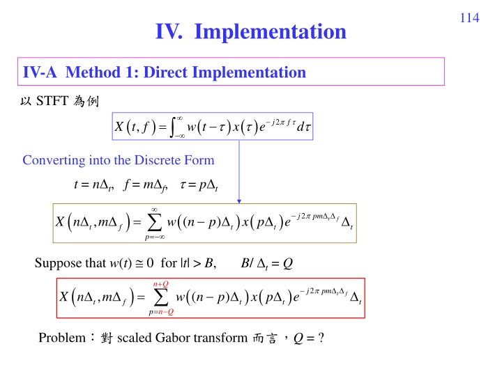
114 IV. Implementation IV-A Method 1: Direct Implementation STFT ( ) ( ) ( ) x = 2 j f , X t f w t e d Converting into the Discrete Form t = n t, f = m f, = p t ( ) ( ) ( x p ) 2 j pm = , ( ) X n m w n p e t f t f t t t = p Suppose that w(t) 0 for |t| > B, B/ t= Q ( , n p = n Q + ) ( ) ( x p ) 2 j pm = ( ) X n m w n p e t f t f t t t Q Problem scaled Gabor transform Q = ?
115 Constraint for t(The only constraint for the direct implementation method) To avoid the aliasing effect, t< 1/2 , is the bandwidth of ? There is no constraint for fwhen using the direct implementation method.
116 Four Implementation Methods (1) Direct implementation Complexity: t-axis T sampling points, f-axis F sampling points (2) FFT-based method Complexity: (3) FFT-based method with recursive formula Complexity: (4) Chirp-Z transform method Complexity:
117 (A) Direct Implementation Advantage simple, flexible Disadvantage higher complexity (B) DFT-Based Method Advantage lower complexity Disadvantage with some constraints (C) Recursive Method Advantage Disadvantage (D) Chirp Z Transform Advantage Disadvantage
118 IV-B Method 2: FFT-Based Method t f= 1/N, N = 1/( t f) 2Q +1: ( t f ) Constraints (ii) (iii) 2 mn N 1 N j Y m y n e = Standard form of the DFT = 0 n n Q + ( ) ( ) ( x p ) 2 j pm = , ( ) X n m w n p e t f t f t t t = p n Q t f= 1/N 2 pm N n Q + ( ) j ( ) ( x p ) = , ( ) X n m w n p e t f t t t = n Q p q = p (n Q) p = (n Q)+q 2 ( ) 2 Q n m N qm N 2 Q ( ) j j ( ) ( x q ) = n Q + , ( ) ( ) X n m e w Q q e t f t t t = 0 q
119 Note that the input of the N-point FFT should have N points (others are set to zero). 2 ( ) 2 Q n m N qm N 1 N ( ) j j ( ) , q = p (n Q) p = (n Q)+q = , X n m e x q e 1 t f t = 0 q ( ) ( x n Q ) ( ) = + ( ) ( ) x q w Q q q for 0 q 2Q, where 1 t t x1(q) = 0 for 2Q < q < N. n-Q n-Q+q n+Q Q Q - q -Q k = q-Q 2 ( ) Q n m N ( ) j ( ) ( ) = , X n m e DFT x q 1 t f t ( ) ( x n ) ( ) ( ) = + -Q k Q for 0 q 2Q, ( ) x q w k k where (k = q-Q) 1 t t x q = 0 for 2Q < q < N. 1 (Suppose that w(t) = w(-t))
120 2 ( ) Q n m N ( ) j ( ) ( ) = , X n m e DFT x q 1 t f t ( ) ( x n ) ( ) ( ) -Q k Q (k = q-Q) = + for ( ) x q w k k where 1 t t (Suppose that w(t) = w(-t)) x q = for 2Q < q < N. center 0 1 ( ) x n t ( ) ( ) ( ) x n ( ) x n Q + ( ) x n Q t t t take a segment of the signal ( ) -Q k Q w k t multiplied by the window ( ) ( t w k x n ) ( ) padding N-2Q-1 zeros + ( ) : k x q 1 t 2 ( ) Q n m N ( ) j ( ) ( ) = , X n m e DFT x q 1 t f t
121 2 ( ) Q n m N ( ) j ( ) ( ) = , X n m e DFT x q 1 t f t 2 qm N 1 N j ( ) ( ) = x q e X m (1) Matlab FFT 1 1 = 0 q (2) n 2 ( 2 ( ) 2 ) Q n m N qm N Q n m N 1 N ( ) j j j ( ) ( ) = = , X n (fixed n) m e x q e e X m 1 1 t f t t = 0 q (3) Complexity = ?
122 t = n0 t, (n0+1) t, (n0+2) t, , (n0+T-1) t f = m0 f, (m0+1) f, (m0+2) f, , (m0+F-1) f Step 1: Calculate n0, m0, T, F, N, Q Step 2: n = n0 Step 3: Determine x1(q) Step 4: X1(m) = FFT[x1(q)] Step 5: Convert X1(m) into X( n t, m f) ( , t f X n m X = m = f/ f m1= mod(m, N)+1 for Matlab page 119 m1= m % N ) ( ) ? ? for Python 1 2 qm N 1 N j = ( ) = + X m x q e X m X m N 1 1 1 1 = 0 q Step 6: Set n = n+1 and return to Step 3 until n = n0+T-1.
123 IV-C Method 3: Recursive Method A very fast way for implementing the rec-STFT 2 pm N n Q + ( ) (n n 1 recursive ) j ( ) = , X n m x p e t f t t = ) p n Q ( = ( 1) , X n m t f (1) Calculate X(min(n) t, m f) by the N-point FFT 2 ( ) Q n N m 2 qm N 1 N ( ) 0 j j ( ) , n0= min(n), = , X n m e x q e 0 1 t f t = 0 q ( ) ( ) = + ( ) x q x n Q q for q 2Q, x1(q) = 0 for q > 2Q 1 t (2) Applying the recursive formula to calculate X(n t, m f), n = n0+1~ max(n) ( ( ( x n Q + + ) ( ) ( ) 2 ( n Q = 1) / j m N , ( 1) , ( 1) X n T F m X n m x n Q e t f t f t t ) 2 ( n Q m N + ) / j ) e t t
124 IV-D Method 4: Chirp Z Transform ( ) ( ) ( ) ( ) = j p j m 2 2 2 exp 2 exp exp ( ) exp j pm j p m t f t f t f t f For the STFT n Q + ( ) ( ) ( x p ) 2 j pm = , ( ) X n m w n p e t f t f t t t p n Q = n Q + ( ) ( ) ( x p ) 2 2 2 j m p m ( ) j p j = , ( ) X n m e w n p e e t f t f t f t f t t t p n Q = Step 1 multiplication Step 2 convolution Step 3 multiplication
125 ( ) ( x p ) 2 j p = ( ) x p w n p e n-Q p n+Q t f Step 1 1 t t n Q + x p c m Step 2 c m 2 = j m , X n m p = e t f 2 1 p n Q = Step 3 ( ) 2 j m = , , X n m e X n m t f 2 t f t Step 2 linear convolution Question: Step 2 DFT?
126 Illustration for the Question on Page 124 = [ ] y n [ ] [ ] k h k x n k Case 1 When length(x[n]) = N, length( h[n]) = K, N and K are finite, length(y[n]) = N+K 1, Using the (N+K 1)-point DFTs ( ) Case 2 x[n] has finite length but h[n] has infinite length ????
127 = [ ] y n [ ] [ ] k h k x n k Case 2 x[n] has finite length but h[n] has infinite length x[n] n [n1, n2] N = n2 n1+ 1 h[n] = y[n] ( [ ] y n [ ] [ ] k h k x n k y[n] y[n] n [m1, m2] M = m2 m1+ 1 h[n] ? FFT ?
128 = = [ ] y n [ ] x n [ ] h n [ ] [ ] k h k x n = k n 2 = = [ ] y n [ ] x n [ ] h n [ ] [ x s h n ] s s n = 1 = + + + + + [ ] y n [ ] [ x n h n n + ] [ 1] [ 1] [ 2] [ 2] x n h n n x n h n n 1 1 ] [ 1 1 1 1 [ ] x n h n n 2 2 n = m1 [ y m = + + + + + ] [ ] [ x n h m ] [ 1] [ 1] [ 2] [ 2] n x n h m n x n h m n 1 1 1 [ 1 1 1 1 1 1 1 + ] [ ] x n h m n 2 1 2 n = m2 [ y m = + + + + + ] [ ] [ x n h m ] [ 1] [ 1] [ 2] [ 2] n x n h m n x n h m n 2 1 2 1 1 2 1 1 2 1 + [ ] [ ] x n h m n 2 2 2
129 m1 n2 m1 n1 n 2 = [ ] y n [ ] [ x s h n ] s s n = m1 n2+1 m1 n1+1 1 m1 n2+2 m1 n1+2 n = m1 n s n = m1+1 n s m2 n2 m2 n1 n = m1+2 n s n = m2 n s h[k] k [m1 n2, m2 n1]
130 k [m1 n2, m2 n1] h[k] m2 n1 m1 + n2+ 1 = N + M 1 FFT implementation for Case 2 [ ] [ ] x n x n n = + x n = for n = 0, 1, 2, , N 1 1 1 for n = N, N + 1, N + 2, , L 1 L = N + M 1 1[ ] 0 = + for n = 0, 1, 2, , L 1 [ ] [ ] h n h n m n 1 1 2 ( ) = [ ] [ ] [ ] y n IFFT FFT x n FFT h n 1 1 1 L L L = + for n = m1, m1+1, m1+2, , m2 [ ] y n [ 1] y n m N 1 1
131 IV-E Unbalanced Sampling for STFT and WDF pages 114 and 118 ( ) ( ) ( ) x = 2 j f , X t f w t e d nS Q + ( ) ( ) ( x p ) 2 j pm = , ( ) X n m w nS p e f t f p nS Q = ( w(t) 0 for |t| > B), where t = n t, f = m f, = p , B = Q S = t/ t (sampling interval for the input signal) t(sampling interval for the output t-axis) can be different. However, it is better that S = t/ is an integer.
132 When (1) f= 1/N, (2) N = 1/( f) > 2Q +1: ( f ) (3) < 1/2 , is the bandwidth of ( | { FT w t x ( ) ( ) t x w i.e., when | f | > ) ( )}| = | ( , )| 0 X t f 2 pm N nS Q + ( ) j ( ) ( x p ) = , ( ) X n m w nS p e t f p nS Q = q = p (nS Q) p = (nS Q) + q 2 ( ) 2 Q nS m N qm N 1 N ( ) j j ( ) = , X n m e x q e 1 t f = 0 q ( ) ( x nS ) ( ) x1(q) = 0 for 2Q < q < N. If w(t) = w(-t)) ( ) ( ) ( 1 ( ) x q w k x nS k = + x1(q) = 0 for 2Q < q < N. for 0 q 2Q, = + ( ) ( ) x q w Q q Q q 1 ) for 0 q 2Q, k = q-Q , -Q k Q
133 t = c0 t, (c0+1) t, (c0+2) t, , (c0+ C -1) t = c0S , (c0S+S) , (c0S+2S) , , [c0S+ (C-1)S] , f = m0 f, (m0+1) f, (m0+2) f, , (m0+F-1) f = n0 , (n0+1) , (n0+2) , , (n0+T-1) , S = t/ Step 1: Calculate c0, m0, n0, C, F, T, N, Q Step 2: n = c0 Step 3: Determine x1(q) Step 4: X1(m) = FFT[x1(q)] Step 5: Convert X1(m) into X( n t, m f) Step 6: Set n = n+1 and return to Step 3 until n = c0+ C -1. Complexity = ?
134 IV-F Non-Uniform t (A) t (B) ( , t f X n m X ) ( ) + ( 1) , n m t f n t, (n+1) t sampling interval t1 ( < t1< t, t/ t1 t1/ ) page 131 ( 1 , , t t f X n m X n + + ) ( ) ( ) + 2 , , , ( 1) , m X n m 1 1 t t f t t f ( ) ( ) + + + , , ( 1) , X n k m X n k m (C) 1 1 t t f t t f sampling interval t2 ( < t2< t1, t1/ t2 t2/ )
135 Gabor transform of a music signal 1000 900 800 700 600 500 400 300 200 100 0 0.2 0.4 0.6 0.8 1 1.2 1.4 1.6 = 1/44100 ( 44100 1.6077 sec + 1 = 70902 )
136 (A) Choose t= running time = out of memory (2008 ) 15.262140 sec (2022 ) (B) Choose t= 0.01 = 441 (1.6/0.01 + 1 = 161 points) running time = 1.0940 sec (2008 ) 0.041053 sec (2022 ) (C) Choose the non-uniform sampling points on the t-axis as t = 0, 0.01, 0.02, 0.03, 0.04, 0.05, 0.1, 0.15, 0.2, 0.4, 0.45, 046, 0.47, 0.48, 0.49, 0.5, 0.51, 0.52, 0.53, 0.54, 0.55, 0.6, 0.8, 0.85, 0.9, 0.95, 0.96, 0.97, 0.98, 0.99, 1, 1.01, 1.02, 1.03, 1.04, 1.05, 1.1, 1.15, 1.2, 1.4, 1.6 (41 points) intervals: 0.2 0.05 0.01 running time = 0.2970 sec (2008 ) 0.010594 sec (2022 )
137 with adaptive output sampling intervals
138 Dirac Delta Function ( ) f = 2 j t f e dt (1) ( ) t ( ) at = (2) a (scaling property) ( g f ) ( ) ( ) 1 g f t g f = = 2 ( ) j ( ) e dt f f (3) n n n where fnare the zeros of g(f) ( ) ( y t ( ) ) = , , t t dt y t (sifting property I) (4) 0 0 ( ) ( y t ( ) ( y t ) ) = (5) , , t t t t (sifting property II) 0 0 0


