Evolution of Metrics in Software Testing

Topics in Metrics for
Software Testing

Quantification
•
One of the characteristics of a maturing
discipline is the replacement of art by
science.
•
Early physics was dominated by
philosophical discussions with no
attempt to quantify things.
•
Quantification was impossible until the
right questions were asked.
Quantification (Cont’d)
•
Computer Science is slowly following
the quantification path.
•
There is skepticism because so much of
what we want to quantify it tied to erratic
human behavior.
Software quantification
•
Software Engineers are still counting
lines of code.
•
This popular metric is highly inaccurate
when used to predict:
–
costs
–
resources
–
schedules
Science begins with
quantification
•
Physics needs measurements for time,
mass, etc.
•
Thermodynamics needs measurements
for temperature.
•
The “size” of software is not obvious.
•
We need an objective measure of
software size.
Software quantification
•
Lines of Code (LOC) is not a good measure
software size.
•
In software testing we need a notion of size
when comparing two testing strategies.
•
The number of tests should be normalized to
software size, for example:
–
S
t
r
a
t
e
g
y
A
n
e
e
d
s
1
.
4
t
e
s
t
s
/
u
n
i
t
s
i
z
e
.
Asking the right questions
•
When can we stop testing?
•
How many bugs can we expect?
•
Which testing technique is more effective?
•
Are we testing hard or smart?
•
Do we have a strong program or a weak test
suite?
•
Currently, we are unable to answer these
questions satisfactorily.
Lessons from physics
•
Measurements lead to Empirical Laws
which lead to Physical Laws.
•
E.g.,
Kepler’s measurements of
planetary movement lead to Newton’s
Laws which lead to Modern Laws of
physics.
Lessons from physics (Cont’d)
•
The metrics we are about to discuss
aim at getting empirical laws that relate
program size to:
–
expected number of bugs
–
expected number of tests required to find
bugs
–
testing technique effectiveness
Metrics taxonomy
•
L
i
n
g
u
i
s
t
i
c
M
e
t
r
i
c
s
:
B
a
s
e
d
o
n
m
e
a
s
u
r
i
n
g
p
r
o
p
e
r
t
i
e
s
o
f
p
r
o
g
r
a
m
t
e
x
t
w
i
t
h
o
u
t
i
n
t
e
r
p
r
e
t
i
n
g
w
h
a
t
t
h
e
t
e
x
t
m
e
a
n
s
.
–
E.g.,
LOC.
•
S
t
r
u
c
t
u
r
a
l
M
e
t
r
i
c
s
:
B
a
s
e
d
o
n
s
t
r
u
c
t
u
r
a
l
r
e
l
a
t
i
o
n
s
b
e
t
w
e
e
n
t
h
e
o
b
j
e
c
t
s
i
n
a
p
r
o
g
r
a
m
.
–
E.g.,
number of nodes and links in a control
flowgraph.
Lines of code (LOC)
•
LOC is used as a measure of software
complexity.
•
This metric is just as good as source listing
weight if we assume consistency w.r.t. paper
and font size.
•
Makes as much sense (or nonsense) to say:
–
“This is a 2 pound program”
•
as it is to say:
–
“This is a 100,000 line program.”
Lines of code paradox
•
P
a
r
a
d
o
x
:
I
f
y
o
u
u
n
r
o
l
l
a
l
o
o
p
,
y
o
u
r
e
d
u
c
e
t
h
e
c
o
m
p
l
e
x
i
t
y
o
f
y
o
u
r
s
o
f
t
w
a
r
e
.
.
.
•
Studies show that there is a linear
relationship between LOC and error rates for
small programs (
i.e.,
LOC < 100).
•
The relationship becomes non-linear as
programs increases in size.
Halstead’s program length
Example of program length
48
7
log
7
+
9
log
9
=
H
1.0)
1,
x,
z,
pow,
0,
(y,
7
=
n
/)
(minus),
-
*,
=,
!
while,
(sign),
=,-
<,
(if,
9
=
n
2
2
2
1
if (y < 0)
pow = - y;
else
pow = y;
z = 1.0;
while (pow != 0) {z = z * x;
pow = pow - 1;
}
if (y < 0)
z = 1.0 / z;
Example of program length
48
7
log
7
+
9
log
9
=
H
temp)
list,
k,
last,
N,
1,
(j,
7
=
n
if)
>,
[],
+,
-,
+,
+
<,
=,
(for,
9
=
n
2
2
2
1
for ( j=1; j<N; j++) {last = N - j + 1;
for (k=1; k <last; k ++) { if (list[k] > list[k+1]) {temp = list[k];
list[k] = list[k+1];
list[k+1] = temp;
}
}
}
Halstead’s bug prediction
How good are
Halstead’s metrics?
•
The validity of the metric has been
confirmed experimentally many times,
independently, over a wide range of
programs and languages.
•
Lipow compared actual to predicted bug
counts to within 8% over a range of
program sizes from 300 to 12,000
statements.
Structural metrics
•
Linguistic complexity is ignored.
•
Attention is focused on control-flow and
data-flow complexity.
•
Structural metrics are based on the
properties of flowgraph models of
programs.
Cyclomatic complexity
•
McCabe’s Cyclomatic complexity is
defined as: M = L - N + 1
•
L = number of links in the flowgraph
•
N = number of nodes in the flowgraph
Property of McCabe’s metric
•
The complexity of several graphs
considered together is equal to the sum
of the individual complexities of those
graphs.
Cyclomatic complexity
heuristics
•
To compute Cyclomatic complexity of a
flowgraph with a single entry and a single
exit:
•
N
o
t
e
:
–
Count n-way case statements as
N
binary
decisions.
–
Count looping as a single binary decision.
Applying cyclomatic complexity to
evaluate test plan completeness
•
Count how many test cases are intended to
provide branch coverage.
•
If the number of test cases <
M
then one of
the following may be true:
–
You haven’t calculated
M
correctly.
–
Coverage isn’t complete.
–
Coverage is complete but it can be done with
more but simpler paths.
–
It might be possible to simplify the routine.
Warning
•
Use the relationship between
M
and the
number of covering test cases as a
guideline not an immutable fact.
When is the creation of a
subroutine cost effective?
•
Break Even Point
occurs when the total
complexities are equal:
•
The break even point is independent of
the main routine’s complexity.
Example
•
If the typical number of calls to a
subroutine is 1.1 (k=1.1), the subroutine
being called must have a complexity of
11 or greater if the net complexity of the
program is to be reduced.
Cost effective subroutines
(Cont’d)
Cost effective subroutines
(Cont’d)
Relationship plotted as a function
•
Note that the function does not make sense
for values of 0 < k < 1 because Mc < 0!
•
Therefore we need to mention that k > 1.
0
1
1
Mc
k
How good is M?
•
A military software project applied the metric
and found that routines with
M
> 10 (23% of
all routines) accounted for 53% of the bugs.
•
Also, of 276 routines, the ones with
M
> 10
had 21% more errors per LOC than those
with
M
<= 10.
•
McCabe advises partitioning routines with
M
> 10.
Pitfalls
•
if ... then ... else
has the same
M
as a
loop!
•
case
statements, which are highly
regular structures, have a high
M
.
•
W
a
r
n
i
n
g
:
M
c
C
a
b
e
’
s
m
e
t
r
i
c
s
h
o
u
l
d
b
e
u
s
e
d
a
s
a
r
u
l
e
o
f
t
h
u
m
b
a
t
b
e
s
t
.
Rules of thumb based on M
•
Bugs/LOC increases discontinuously for
M
> 10
•
M
is better than LOC in judging life-cycle
efforts.
•
Routines with a high
M
(say > 40) should be
scrutinized.
•
M
establishes a useful lower-bound rule of
thumb for the number of test cases required
to achieve branch coverage.
Software testing
process metrics
•
Bug tracking tools enable the extraction of
several useful metrics about the software and
the testing process.
•
Test managers can see if any trends in the
data show areas that:
–
may need more testing
–
are on track for its scheduled release date
•
Examples of software testing process metrics:
–
Average number of bugs per tester per day
–
Number of bugs found per module
–
The ratio of Severity 1 bugs to Severity 4 bugs
–
…
Example queries applied to a
bug tracking database
•
What areas of the software have the most
bugs? The fewest bugs?
•
How many resolved bugs are currently
assigned to John?
•
Mary is leaving for vacation soon. How many
bugs does she have to fix before she leaves?
•
Which tester has found the most bugs?
•
What are the open Priority 1 bugs?
Example data plots
•
Number of bugs versus:
–
fixed bugs
–
deferred bugs
–
duplicate bugs
–
non-bugs
•
Number of bugs versus each major functional
area of the software:
–
GUI
–
documentation
–
floating-point arithmetic
–
etc
Example data plots (cont’d)
•
Bugs opened versus date opened over time:
–
This view can show:
•
bugs opened each day
•
cumulative opened bugs
•
On the same plot we can plot resolved bugs,
closed bugs, etc to compare the trends.
You now know …
•
… the importance of quantification
•
… various software metrics
•
… various software testing process
metrics and views
The evolution of metrics in software testing involves the transition from subjective discussions to quantifiable measurements, mirroring the development of mature disciplines like physics. While early software engineering relied on simplistic measures like lines of code, the need for more sophisticated metrics is becoming apparent. By asking the right questions and learning lessons from physics, we can strive to establish empirical laws that link program size to important testing considerations.

Download Presentation

Please find below an Image/Link to download the presentation.
The content on the website is provided AS IS for your information and personal use only. It may not be sold, licensed, or shared on other websites without obtaining consent from the author. Download presentation by click this link. If you encounter any issues during the download, it is possible that the publisher has removed the file from their server.
E N D
Presentation Transcript
Topics in Metrics for Software Testing
Quantification One of the characteristics of a maturing discipline is the replacement of art by science. Early physics was dominated by philosophical discussions with no attempt to quantify things. Quantification was impossible until the right questions were asked.
Quantification (Contd) Computer Science is slowly following the quantification path. There is skepticism because so much of what we want to quantify it tied to erratic human behavior.
Software quantification Software Engineers are still counting lines of code. This popular metric is highly inaccurate when used to predict: costs resources schedules
Science begins with quantification Physics needs measurements for time, mass, etc. Thermodynamics needs measurements for temperature. The size of software is not obvious. We need an objective measure of software size.
Software quantification Lines of Code (LOC) is not a good measure software size. In software testing we need a notion of size when comparing two testing strategies. The number of tests should be normalized to software size, for example: Strategy A needs 1.4 tests/unit size.
Asking the right questions When can we stop testing? How many bugs can we expect? Which testing technique is more effective? Are we testing hard or smart? Do we have a strong program or a weak test suite? Currently, we are unable to answer these questions satisfactorily.
Lessons from physics Measurements lead to Empirical Laws which lead to Physical Laws. E.g., Kepler s measurements of planetary movement lead to Newton s Laws which lead to Modern Laws of physics.
Lessons from physics (Contd) The metrics we are about to discuss aim at getting empirical laws that relate program size to: expected number of bugs expected number of tests required to find bugs testing technique effectiveness
Metrics taxonomy Linguistic Metrics: Based on measuring properties of program text without interpreting what the text means. E.g., LOC. Structural Metrics: Based on structural relations between the objects in a program. E.g., number of nodes and links in a control flowgraph.
Lines of code (LOC) LOC is used as a measure of software complexity. This metric is just as good as source listing weight if we assume consistency w.r.t. paper and font size. Makes as much sense (or nonsense) to say: This is a 2 pound program as it is to say: This is a 100,000 line program.
Lines of code paradox Paradox: If you unroll a loop, you reduce the complexity of your software ... Studies show that there is a linear relationship between LOC and error rates for small programs (i.e., LOC < 100). The relationship becomes non-linear as programs increases in size.
Example of program length n = 9 (if, <, =,- (sign), while, if (y < 0) pow = - y; else pow = y; z = 1.0; while (pow != 0) { z = z * x; pow = pow - 1; } if (y < 0) z = 1.0 / z; 1 ! =, *, - (minus), /) n = 7 (y, 0, pow, z, x, 1, 1.0) 2 H = 9 log 9 + 7 log 7 48 2 2
Example of program length for ( j=1; j<N; j++) { last = N - j + 1; for (k=1; k <last; k ++) { if (list[k] > list[k+1]) { temp = list[k]; list[k] = list[k+1]; list[k+1] = temp; } } } n = 9 (for, =, <, + +, -, +, [], >, if) 1 n = 7 (j, 1, N, last, k, list, temp) 2 H = 9 log 9 + 7 log 7 48 2 2
How good are Halstead s metrics? The validity of the metric has been confirmed experimentally many times, independently, over a wide range of programs and languages. Lipow compared actual to predicted bug counts to within 8% over a range of program sizes from 300 to 12,000 statements.
Structural metrics Linguistic complexity is ignored. Attention is focused on control-flow and data-flow complexity. Structural metrics are based on the properties of flowgraph models of programs.
Cyclomatic complexity McCabe s Cyclomatic complexity is defined as: M = L - N + 1 L = number of links in the flowgraph N = number of nodes in the flowgraph
Property of McCabes metric The complexity of several graphs considered together is equal to the sum of the individual complexities of those graphs.
Cyclomatic complexity heuristics To compute Cyclomatic complexity of a flowgraph with a single entry and a single exit: Note: Count n-way case statements as N binary decisions. Count looping as a single binary decision.
Applying cyclomatic complexity to evaluate test plan completeness Count how many test cases are intended to provide branch coverage. If the number of test cases < M then one of the following may be true: You haven t calculated M correctly. Coverage isn t complete. Coverage is complete but it can be done with more but simpler paths. It might be possible to simplify the routine.
Warning Use the relationship between M and the number of covering test cases as a guideline not an immutable fact.
When is the creation of a subroutine cost effective? Break Even Point occurs when the total complexities are equal: The break even point is independent of the main routine s complexity.
Example If the typical number of calls to a subroutine is 1.1 (k=1.1), the subroutine being called must have a complexity of 11 or greater if the net complexity of the program is to be reduced.
Cost effective subroutines (Cont d)
Cost effective subroutines (Cont d)
Relationship plotted as a function Mc 1 0 1 k Note that the function does not make sense for values of 0 < k < 1 because Mc < 0! Therefore we need to mention that k > 1.
How good is M? A military software project applied the metric and found that routines with M > 10 (23% of all routines) accounted for 53% of the bugs. Also, of 276 routines, the ones with M > 10 had 21% more errors per LOC than those with M <= 10. McCabe advises partitioning routines with M > 10.
Pitfalls if ... then ... else has the same M as a loop! case statements, which are highly regular structures, have a high M. Warning:McCabe s metric should be used as a rule of thumb at best.
Rules of thumb based on M Bugs/LOC increases discontinuously for M > 10 M is better than LOC in judging life-cycle efforts. Routines with a high M (say > 40) should be scrutinized. M establishes a useful lower-bound rule of thumb for the number of test cases required to achieve branch coverage.
Software testing process metrics Bug tracking tools enable the extraction of several useful metrics about the software and the testing process. Test managers can see if any trends in the data show areas that: may need more testing are on track for its scheduled release date Examples of software testing process metrics: Average number of bugs per tester per day Number of bugs found per module The ratio of Severity 1 bugs to Severity 4 bugs
Example queries applied to a bug tracking database What areas of the software have the most bugs? The fewest bugs? How many resolved bugs are currently assigned to John? Mary is leaving for vacation soon. How many bugs does she have to fix before she leaves? Which tester has found the most bugs? What are the open Priority 1 bugs?
Example data plots Number of bugs versus: fixed bugs deferred bugs duplicate bugs non-bugs Number of bugs versus each major functional area of the software: GUI documentation floating-point arithmetic etc
Example data plots (contd) Bugs opened versus date opened over time: This view can show: bugs opened each day cumulative opened bugs On the same plot we can plot resolved bugs, closed bugs, etc to compare the trends.
You now know the importance of quantification various software metrics various software testing process metrics and views


")


")

")


")