Decision Trees in R

Decision trees are a popular technique for data classification that involve splitting attributes to make predictions. The examples provided showcase how decision trees work in R, depicting various scenarios and outcomes based on different attributes and conditions. These illustrations offer a practical understanding of decision tree classification tasks, tree induction algorithms, training datasets, and model application to test data. By applying decision trees, data can be effectively classified by partitioning attribute space, with clear representation of class labels in the leaf nodes for informed decision-making.

Download Presentation

Please find below an Image/Link to download the presentation.
The content on the website is provided AS IS for your information and personal use only. It may not be sold, licensed, or shared on other websites without obtaining consent from the author.If you encounter any issues during the download, it is possible that the publisher has removed the file from their server.
You are allowed to download the files provided on this website for personal or commercial use, subject to the condition that they are used lawfully. All files are the property of their respective owners.
The content on the website is provided AS IS for your information and personal use only. It may not be sold, licensed, or shared on other websites without obtaining consent from the author.
E N D
Presentation Transcript
Decision Trees in R Arko Barman With additions and modifications by Ch. Eick For COSC 3337
Example of a Decision Tree Splitting Attributes Tid Refund Marital Status Taxable Income Cheat No 1 Yes Single 125K Refund No 2 No Married 100K Yes No No 3 No Single 70K No 4 Yes Married 120K NO MarSt Yes 5 No Divorced 95K Married Single, Divorced No 6 No Married 60K TaxInc NO No 7 Yes Divorced 220K < 80K > 80K Yes 8 No Single 85K No 9 No Married 75K YES NO Yes 10 No Single 90K 10 Model: Decision Tree Training Data
Another Example of Decision Tree Single, Divorced MarSt Married Tid Refund Marital Status Taxable Income Cheat NO Refund No 1 Yes Single 125K No Yes No 2 No Married 100K NO TaxInc No 3 No Single 70K < 80K > 80K No 4 Yes Married 120K Yes 5 No Divorced 95K YES NO No 6 No Married 60K No 7 Yes Divorced 220K Yes 8 No Single 85K There could be more than one tree that fits the same data! No 9 No Married 75K Yes 10 No Single 90K 10
Decision Tree Classification Task Tree Induction algorithm Attrib1 Attrib2 Attrib3 Class Tid No 1 Yes Large 125K No 2 No Medium 100K No 3 No Small 70K Induction No 4 Yes Medium 120K Yes 5 No Large 95K No 6 No Medium 60K Learn Model No 7 Yes Large 220K Yes 8 No Small 85K No 9 No Medium 75K Yes 10 No Small 90K Model 10 Training Set Apply Model Decision Tree Attrib1 Attrib2 Attrib3 Class Tid ? 11 No Small 55K ? 12 Yes Medium 80K Deduction ? 13 Yes Large 110K ? 14 No Small 95K ? 15 No Large Test Set 67K 10
Apply Model to Test Data Test Data Start from the root of tree. Refund Marital Taxable Income Cheat Status No Married 80K ? Refund 10 Yes No NO MarSt Married Single, Divorced TaxInc NO < 80K > 80K YES NO
Apply Model to Test Data Test Data Refund Marital Taxable Income Cheat Status No Married 80K ? Refund 10 Yes No NO MarSt Married Single, Divorced TaxInc NO < 80K > 80K YES NO
Decision Trees Used for classifying data by partitioning attribute space Leaf nodes contain class labels, representing classification decisions and intermediate nodes represent traffic signs . Keeps splitting nodes based on split criterion, such as GINI index, information gain or entropy Tries to find axis-parallel decision boundaries for numerical attributes and uses n-way splits for a symbolic attribute with n values. Pruning necessary to avoid overfitting
Decision Trees in R mydata<-data.frame(iris) attach(mydata) library(rpart) model<-rpart(Species ~ Sepal.Length + Sepal.Width + Petal.Length + Petal.Width, data=mydata, method="class") plot(model) text(model,use.n=TRUE,all=TRUE,cex=0.8)
Decision Trees in R library(tree) model1<-tree(Species ~ Sepal.Length + Sepal.Width + Petal.Length + Petal.Width, data=mydata, method="class", split="gini") plot(model1) text(model1,all=TRUE,cex=0.6)
Decision Trees in R library(party) model2<-ctree(Species ~ Sepal.Length + Sepal.Width + Petal.Length + Petal.Width, data=mydata) plot(model2)
Hyperparameter Tuning and Pruning: More about Decision Trees in R with rpart | by Dima Diachkov | Data And Beyond | Medium Controlling number of nodes This is just an example. You can come up with better or more efficient methods! library(tree) mydata<-data.frame(iris) attach(mydata) model1<-tree(Species ~ Sepal.Length + Sepal.Width + Petal.Length + Petal.Width, data=mydata, method="class", control = tree.control(nobs = 150, mincut = 10)) plot(model1) text(model1,all=TRUE,cex=0.6) predict(model1,iris) Note how the number of nodes is reduced by increasing the minimum number of observations in a child node!
Controlling number of nodes This is just an example. You can come up with better or more efficient methods! model2<-ctree(Species ~ Sepal.Length + Sepal.Width + Petal.Length + Petal.Width, data = mydata, controls = ctree_control(maxdepth=2)) plot(model2) Note that setting the maximum depth to 2 has reduced the number of nodes!
http://data.princeton.edu/R/linearmodels.html Linear Models in R abline() adds one or more straight lines to a plot lm() function to fit linear regression model x1<-c(1:5,1:3) x2<-c(2,2,2,3,6,7,5,1) abline(lm(x2~x1)) title('Regression of x2 on X1') plot(x1,x2) abline(lm(x2~x1)) title('Regression of x2 on + x1') s<-lm(x2~x1) lm(x1~x2) abline(1,2)
Scaling and Z-Scoring Datasets http://stat.ethz.ch/R-manual/R- patched/library/base/html/scale.html s<-scale(iris[1:4]) mean(s[,1]) sd(s[,1]) t<-scale(s, center=c(5,5,5,5), scale=FALSE) #subtracts the mean-vector and additionally (5,5,5,5) and does not divide by the standard deviation. https://archive.ics.uci.edu/ml/datasets/banknote +authentication
NAs and Statistical Summaries > #also see: http://thomasleeper.com/Rcourse/Tutorials/NAhandling.html > #Author: Christoph Eick; February 9, 2018. > #Dealing with NA's > a<-c(1,NA,4,7) > sd(a) [1] NA > sd(a, na.rm=TRUE) [1] 3 > mean(a, na.rm=TRUE) [1] 4 > cor(iris[1:4]) Sepal.Length Sepal.Width Petal.Length Petal.Width Sepal.Length 1.0000000 -0.1175698 0.8717538 0.8179411 Sepal.Width -0.1175698 1.0000000 -0.4284401 -0.3661259 Petal.Length 0.8717538 -0.4284401 1.0000000 0.9628654 Petal.Width 0.8179411 -0.3661259 0.9628654 1.0000000
NAs and Statistical Summaries II > a<-c(NA,NA,5,6,7,8, 9, 10, 12) > b<-c(1,2,NA,NA,4,4, 7, 2, 4) > c<-c(3,3,1,6,NA,NA, 5, -4, -6) > x<-data.frame(a,b,c) > x a b c 1 NA 1 3 2 NA 2 3 3 5 NA 1 4 6 NA 6 5 7 4 NA 6 8 4 NA 7 9 7 5 8 10 2 -4 9 12 4 -6 > cor(x) a b c a 1 NA NA b NA 1 NA c NA NA 1 > cor(x, use="complete.obs") a b c a 1.0000000 -0.4335550 -0.8565648 b -0.4335550 1.0000000 0.8363851 c -0.8565648 0.8363851 1.0000000 > cor(x, use="pairwise.complete.obs") a b c a 1.0000000 -0.1598405 -0.6981545 b -0.1598405 1.0000000 0.1892828 c -0.6981545 0.1892828 1.0000000 > cov(x, use="pairwise.complete.obs") #I recommend using "pairwise.complete.obs", but this can also lead to problems: http://bwlewis.github.io/covar/missing.html