Decision Diagrams for Sequencing and Scheduling Techniques
This research explores the application of decision diagrams for optimization problems, particularly in sequencing and scheduling. The study delves into novel techniques for discrete optimization problems, providing insights into decision diagram definitions and their practical applications. The diagrams serve as graphical representations of solution sets to facilitate problem-solving processes. With a focus on decision diagrams for sequencing and scheduling, the research offers valuable contributions to the field of operations research and optimization.

Download Presentation

Please find below an Image/Link to download the presentation.
The content on the website is provided AS IS for your information and personal use only. It may not be sold, licensed, or shared on other websites without obtaining consent from the author.If you encounter any issues during the download, it is possible that the publisher has removed the file from their server.
You are allowed to download the files provided on this website for personal or commercial use, subject to the condition that they are used lawfully. All files are the property of their respective owners.
The content on the website is provided AS IS for your information and personal use only. It may not be sold, licensed, or shared on other websites without obtaining consent from the author.
E N D
Presentation Transcript
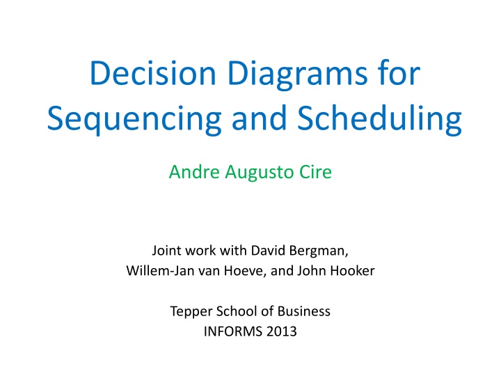
Decision Diagrams for Sequencing and Scheduling Andre Augusto Cire Joint work with David Bergman, Willem-Jan van Hoeve, and John Hooker Tepper School of Business INFORMS 2013
Decision Diagrams for Optimization Novel techniques for discrete optimization problems C., van Hoeve: Multivalued Decision Diagrams for Sequencing Problems, Operations Research, to appear. Bergman, C., van Hoeve, Hooker: Optimization Bounds from Binary Decision Diagrams. INFORMS J. Computing, to appear. C., van Hoeve: MDD Propagation for Disjunctive Scheduling, ICAPS 2012 Bergman, C., van Hoeve, Hooker: Variable Ordering for the Application of BDDs to the Maximum Independent Set Problem. CPAIOR 2012: 34-49 Bergman, C., van Hoeve, Hooker: Decision Diagrams for Discrete Optimization. Under review, 2013. ... 2
Outline Definition of a decision diagram Application to timetable problems Application to disjunctive scheduling 3
What is a decision diagram? In our context: A decision diagram is a graphical representation of a set of solutions to a problem 4
max i xi x1 + x2 x3 + x6 x1 + x4 + x5 1 x4 + x5 + x6 1 1 1 x1, , x6 {0,1} 5
: 0 r : 1 x1 max i xi x1 + x2 x3 + x6 x1 + x4 + x5 1 x4 + x5 + x6 1 1 1 x2 x3 x1, , x6 {0,1} x4 Layers: variables x5 Arc labels: variable values Paths from root to terminal: solutions x6 t 6
: 0 r : 1 x1 max i xi x1 + x2 x3 + x6 x1 + x4 + x5 1 x4 + x5 + x6 1 1 1 x2 x3 x1, , x6 {0,1} x4 Layers: variables x5 Arc labels: variable values Paths from root to terminal: solutions x6 t 7
: 0 r : 1 x1 max i xi x1 + x2 x3 + x6 x1 + x4 + x5 1 x4 + x5 + x6 1 1 1 x2 x3 x1, , x6 {0,1} x4 Arc weights: contribution to the objective function x5 Optimal solution: longest path from root to terminal x6 t 8
: 0 r : 1 x1 max i xi x1 + x2 x3 + x6 x1 + x4 + x5 1 x4 + x5 + x6 1 1 1 x2 x3 x1, , x6 {0,1} x4 Arc weights: contribution to the objective function x5 Optimal solution: longest path from root to terminal x6 t 9
Issue Exactly representing all solutions requires exponentially-sized diagrams Alternative: Limit its size to obtain a relaxation of the set of solutions instead Limit the width of the diagram Strength is controlled by the width 10
max i xi x1 + x2 x3 + x6 x1 + x4 + x5 1 x4 + x5 + x6 1 1 1 x1 x2 x1, , x6 {0,1} x3 x4 x5 x6 Exact Width = 4 Relaxed Width = 3 11
max i xi x1 + x2 x3 + x6 x1 + x4 + x5 1 x4 + x5 + x6 1 1 1 x1 x2 x1, , x6 {0,1} x3 x4 x5 x6 Exact Width = 4 Relaxed Width = 3 12
max i xi x1 + x2 x3 + x6 x1 + x4 + x5 1 x4 + x5 + x6 1 1 1 x1 x2 x1, , x6 {0,1} x3 x4 x5 Relaxation provides an upper bound of 4 x6 Exact Width = 4 Relaxed Width = 3 13
Relaxed Diagrams Provide bounds on the objective function They can also be used for inference Deduction of new constraints 14
Constructing Relaxed Diagrams Incremental refinement Constraints are processed one at a time Refine phase Filter phase 15
r : 0 : 1 x1 max i xi x1 + x2 x3 + x6 x1 + x4 + x5 1 x4 + x5 + x6 1 x1, , x6 {0,1} x2 1 1 x3 x4 x5 Maximum Width: 2 x6 t 16
r : 0 Refine: constraint selects a node to split : 1 x1 max i xi x1 + x2 x3 + x6 x1 + x4 + x5 1 x4 + x5 + x6 1 x1, , x6 {0,1} x2 1 1 x3 x4 x5 Maximum Width: 2 x6 t 17
r : 0 Refine: constraint selects a node to split : 1 x1 max i xi x1 + x2 x3 + x6 x1 + x4 + x5 1 x4 + x5 + x6 1 x1, , x6 {0,1} x2 1 1 x3 x4 x5 Maximum Width: 2 x6 t 18
r : 0 Refine: constraint selects a node to split : 1 x1 max i xi x1 + x2 x3 + x6 x1 + x4 + x5 1 x4 + x5 + x6 1 x1, , x6 {0,1} x2 1 1 x3 x4 x5 Maximum Width: 2 x6 t 19
r : 0 Filter: remove infeasible arcs : 1 x1 max i xi x1 + x2 x3 + x6 x1 + x4 + x5 1 x4 + x5 + x6 1 x1, , x6 {0,1} x2 1 1 x3 x4 x5 Maximum Width: 2 x6 t 20
r : 0 Filter: remove infeasible arcs : 1 x1 max i xi x1 + x2 x3 + x6 x1 + x4 + x5 1 x4 + x5 + x6 1 x1, , x6 {0,1} x2 1 1 x3 x4 x5 Maximum Width: 2 x6 t 21
r : 0 Filter: remove infeasible arcs : 1 x1 max i xi x1 + x2 x3 + x6 x1 + x4 + x5 1 x4 + x5 + x6 1 x1, , x6 {0,1} x2 1 1 x3 x4 x5 Maximum Width: 2 x6 t 22
r : 0 Move to the next constraint and repeat... : 1 x1 max i xi x1 + x2 x3 + x6 x1 + x4 + x5 1 x4 + x5 + x6 1 x1, , x6 {0,1} x2 1 1 x3 x4 x5 Maximum Width: 2 x6 t 23
Key Observation Constraints can be highly-structured Suitable to scheduling Two application examples Timetable problems Disjunctive scheduling 24
Timetable Problems Example: Allocate work days and rest days for an employee throughout the week Each employee must have at least one rest day for every three consecutive days Sequence constraint 25
Linear formulation: Decision variable: - xi: 1 if employee works on day i, 0 otherwise sun mon tue wed thu fri sat x1 x2 x3 x4 x5 x6 x7 x4+x5+x6 2 x5+x6+x7 2 x2+x3+x4 2 x3+x4+x5 2 x1+x2+x3 2 x1+x2+x3 2 x2+x3+x4 2 Typical sequence linear model x3+x4+x5 2 x4+x5+x6 2 x5+x6+x7 2 26
: 0 Diagram Representation : 1 r sun mon tue wed thu x1 x1 x2 x3 x4 x5 x2 Layers: work allocation variables x3 Variable ordering in the diagram corresponds to day sequence x4 x5 t 27
: 0 Filtering : 1 (0, 0) r x1 State information for each node: Minimum and maximum work days up to that node (1, 1) (0, 0) x2 (1, 1) (2, 2) (0, 0) x3 (1, 1) x1 + x2 + x3 2 (2, 3) (0, 2) x4 (1, 4) (1, 1) (0, 2) x5 t (0, 5) 28
: 0 (0, 0) : 1 r x1 (1, 1) (0, 0) 0 ?1 2 x2 2 0 ?=1 ?? 2 (2, 2) (1, 1) (0, 0) x3 3 1 ?=1 ?? 2 (2, 2) (1, 1) (2, 2) x4 4 1 ?=1 ?? 3 (1, 1) (2, 2) (3, 3) x5 3 2 ?=1 ?? 4 t (2, 4) 29
Experimental Results Hard randomly generated instances 50 days 5 sequence constraints Inference was incorporated into a state-of- the-art constraint-based scheduler (ILOG CP Optimizer) New type of global constraint 30
Results 31
Disjunctive Scheduling Sequencing and scheduling of activities on a resource 0 2 3 4 1 Activities Processing time: pi Release time: ri Deadline: di Activity 1 Activity 2 Activity 3 Resource Nonpreemptive Process one activity at a time 32
Diagram Representation Natural representation as permutation diagram Every solution can be written as a permutation 1, 2 , 3, , n : activity sequencing in the resource Schedule is implied by a sequence: ??????? ??????? 1+ ??? 1 ? = 2, ,? 34
Diagram Representation Act ri 0 pi 2 di 3 1 1 {1} 2 4 2 9 3 3 3 8 2 {3} {2} Path {1} {3} {2} : 3 0 start1 1 {2} {3} 6 start2 7 3 start3 5 35
Filtering r 1 {1,2} {3} Example of state information: Earliest starting time {3} 2 {1} {1,2} {1} 3 {2} {3} 4 {1,3,5, } 36
Filtering: Earliest Start Time 0 r Assume all release dates are zero, and: 1 {1,2} {3} 5 2 Act pi 2 di 12 {3} 2 {1} {1,2} 8 1 2 3 6 7 4 {1} 3 5 18 3 {2} {3} Node labels: 4 Earliest Start Time {1,3,5, } 37
Filtering: Earliest Start Time 0 r Assume all release dates are zero, and: 1 {1,2} {3} 5 2 Act pi 2 di 12 {3} 2 {1} {1,2} 8 1 2 3 6 7 4 {1} 3 5 18 3 {2} {3} Node labels: 4 Earliest Start Time {1,3,5, } 38
Inference Theorem: Given the exact diagram M, we can deduce all implied activity precedence in polynomial time in the size of M For a node v, : values in all paths from root to u : values in all paths from node u to terminal r ?? ?? i u Precedence relation ? ? holds if and only if for all nodes u in M j Same technique applies to relaxed MDD t 39
Precedence relations can be used to: Guide search As an inference technique Mathematical Programming: linear constraints Constraint-based scheduling: reduce domains Conversely, precedence relations can also be used to filter the permutation diagram 40
Experiments Decision diagram incorporated into IBM ILOG CPLEX CP Optimizer 12.4 (CPO) State-of-the-art constraint based scheduling solver Uses a portfolio of inference techniques and LP relaxation Added as user-defined propagator 41
TSP with Time Windows Dumas/Ascheuer instances - 20-60 jobs - lex search - MDD width: 16 Pure MDD time (s) CPO time (s) 42
Total Tardiness Results MDD-128 MDD-128 MDD-64 MDD-64 MDD-32 MDD-32 CPO MDD-16 MDD-16 CPO total tardiness total weighted tardiness 43
Other results Asymmetric TSP with Precedence Constraints Closed 3 open instances Similar results to more complex problems Example: Machine deterioration 44
Final Remarks New approach for scheduling applications Orders of magnitude speed-ups Bounding mechanism Provide highly-structured information that can be sent to existing solvers 45
Scheduling: Allocation of resources to tasks over time 60 years of research Still a fundamental component in supply chain management and optimization 47
Recent Franz Elderman Award Winners TNT Express, 2012 Network routing and scheduling Netherland Railways, 2008 Timetable Warner Robin Air Logistics, 2006 Allocation of repair tasks ... 48
How are they being solved? Combination of techniques: Specialized Heuristics Large-scale instances, but hard to maintain Mathematical Programming Advanced solvers Constraint-based scheduling Inference Model-based Several problems still hard to model and solve Over-reliance on specialized heuristics 49
Scheduling: Allocation of resources to tasks over time 60 years of research Still a fundamental component in supply chain management and optimization 50