Cyclonic Flow Analysis in Atmospheric Dynamics Study

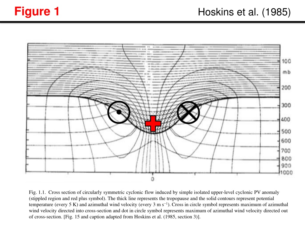
Fig. 1.1.  Cross section of circularly symmetric cyclonic flow induced by simple isolated upper-level cyclonic PV anomaly

(stippled region and red plus symbol). The thick line represents the tropopause and the solid contours represent potential

temperature (every 5 K) and azimuthal wind velocity (

every 3 m s

−1

). Cross in circle symbol represents maximum of azimuthal

wind velocity directed into cross-section and dot in circle symbol represents maximum of azimuthal wind velocity directed out

of cross-section. [Fig. 15 and caption adapted from Hoskins et al. (1985, section 3)].

F

i

g

u

r

e

1

Hoskins et al. (1985)

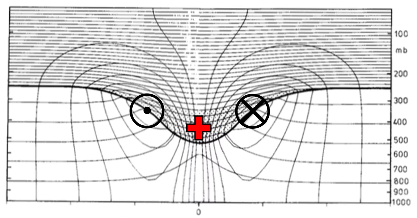
Fig 1.2. 

Analyses for 0000 UTC 30 Nov 1991: (a) DT (1.5-PVU) potential temperature (thin solid, values at and below 342 K

contoured at a 6-K interval, shaded as indicated for values below 294 K) and DT wind speed (thick solid; contour interval, 

15 

m s

−1

;

starting at 

50 

m s

−1

); and (b) DT pressure (thin solid; contour interval, 40 hPa; shaded as indicated for values greater than 480 hPa) and

DT horizontal wind speed [contoured as in (a)].

 Label “TPV” and arrow point to position of TPV. [Fig. 11 and caption adapted from

Pyle et al. (2004)].

F

i

g

u

r

e

2

Pyle et al. (2004)

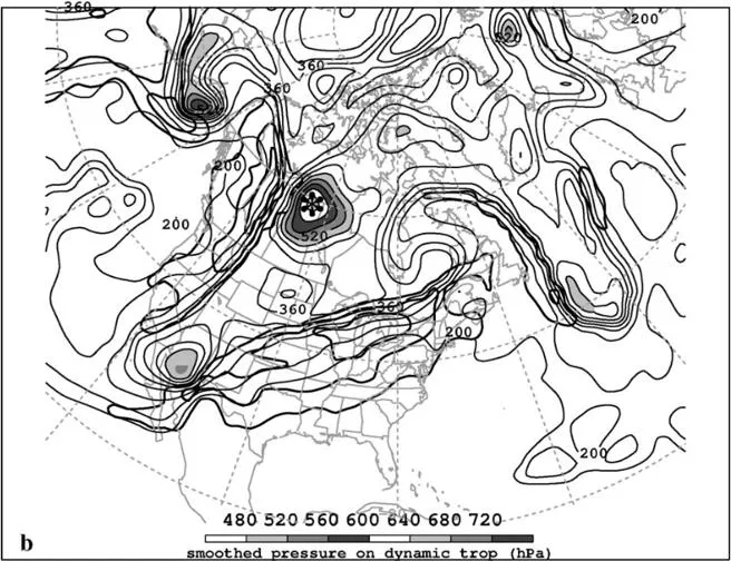
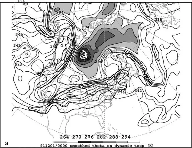
Fig. 2.  Analyses for 0000 UTC 30 Nov 1991: (a) DT (1.5-PVU) potential temperature (thin solid, values at and below 342 K contoured at a

6-K interval, shaded as indicated for values below 294 K) and DT wind speed (thick solid; contour interval, 

15 

m s

−1

; starting at 

50 

m s

−1

);

(b) DT pressure (thin solid; contour interval, 40 hPa; shaded as indicated for values greater than 480 hPa) and DT wind speed [contoured as in

(a)]; (c) 300-hPa geopotential height (thin solid; contour at a 12-dam interval), 300-hPa wind speed [contoured as in (a)], and wind (plotted

using standard convention: pennant, full barb, and half barb denote 25, 5, and 2.5 m s

−1

, respectively); and (d) PV calculated over the 316–

324-K layer (thin solid; contour at a 0.8-PVU interval for values greater than 1.6 PVU, shaded as indicated for values greater than 5.6 PVU)

and wind speed at 320 K [contoured as in (a)]. The position of the DT pressure maximum associated with the TPV of interest is marked with

an asterisk in each panel. 

[Fig. 11 and caption adapted from Pyle et al. (2004)].

F

i

g

u

r

e

2

Pyle et al. (2004)

Fig. 2.  Analyses for 0000 UTC 30 Nov 1991: (a) DT (1.5-PVU) potential temperature (thin solid, values at and below 342 K contoured at a

6-K interval, shaded as indicated for values below 294 K) and DT wind speed (thick solid; contour interval, 

15 

m s

−1

; starting at 

50 

m s

−1

);

(b) DT pressure (thin solid; contour interval, 40 hPa; shaded as indicated for values greater than 480 hPa) and DT wind speed [contoured as in

(a)]; (c) 300-hPa geopotential height (thin solid; contour at a 12-dam interval), 300-hPa wind speed [contoured as in (a)], and wind (plotted

using standard convention: pennant, full barb, and half barb denote 25, 5, and 2.5 m s

−1

, respectively); and (d) PV calculated over the 316–

324-K layer (thin solid; contour at a 0.8-PVU interval for values greater than 1.6 PVU, shaded as indicated for values greater than 5.6 PVU)

and wind speed at 320 K [contoured as in (a)]. The position of the DT pressure maximum associated with the TPV of interest is marked with

an asterisk in each panel.

 Label “TPV” and arrow point to position of TPV.

[Fig. 11 and caption adapted from Pyle et al. (2004)].

F

i

g

u

r

e

2

Pyle et al. (2004)

Fig. 1.3.  Composite west–east cross-TPV section of anomalous (a) temperature (K), (b) v-wind component (m s

−1

), (c) Ertel PV (PVU),

and (d) relative humidity (%). Thick solid black contour is the composite tropopause and thick dashed black contour is the background

tropopause. The 0 contour is denoted by the thin, solid contour. [Fig. 9 and adapted caption from Cavallo and Hakim (2010)].

F

i

g

u

r

e

3

Cavallo and Hakim (2010)

Fig. 1.4.  (a) Skew 

T

–log

p

 diagram of composite

temperature and dewpoint temperature at the TPV

core (solid) and at the background grid point

(dashed). (b) Vortex–background difference plots

of temperature (solid) and relative humidity

(dashed). The plots to the right show the

corresponding PV in (a) and PV anomaly from the

background in (b) in PVUs at the TPV core (solid)

and background grid point (dashed). [Fig. 6 and

adapted caption from Cavallo and Hakim (2010)].

F

i

g

u

r

e

4

Cavallo and Hakim (2010)

Fig. 1.5.  Total number of tropopause cyclonic vortex events occurring in a 2.5°–10° lat–lon box centered at a

point, with a cosine-latitude normalization applied for equal-area weighting [Fig. 2 and adapted caption from

Hakim and Canavan (2005)].

F

i

g

u

r

e

4

Hakim and Canavan (2005)

F

i

g

u

r

e

6

Fig. 1.6.  Tracks of QGPV maxima and time-

mean 500-hPa geopotential height field (black,

contoured every 12 dam) for 17–27 January

1978. Tracks of QGPV maxima (blue dots

represent arctic QGPV maximum and green dots

represents midlatitude QGPV maximum) and

1000–500-hPa thickness minima (black crosses)

involved in the formation of the 1978 Cleveland

Superbomb every 24 h starting 0000 UTC 17

January and ending 0000 UTC 27 January 1978.

Red dot represents the merger of the two QGPV

maxima. [Fig. 3 and caption adapted from Hakim

et al. (1995)].

Hakim et al. (1995)

F

i

g

u

r

e

5

Hoskins et al. (1985)

Fig. 1.7.  A schematic picture of cyclogenesis associated with the arrival of an upper-level cyclonic PV anomaly over a low-level

baroclinic region. In both (a) and (b) solid plus sign indicates location of upper-level cyclonic PV anomaly, solid black contour at the

top represents the tropopause, black contours at bottom represent isentropes at the ground, thick solid arrow represents the cyclonic

circulation induced by upper-level cyclonic PV anomaly at upper-levels, and thin solid arrow represents the cyclonic circulation

induced by upper-level cyclonic PV anomaly at low-levels. In (b) only, open plus sign represents low-level warm temperature

anomaly, thick open arrow represents cyclonic circulation induced by the low-level warm temperature anomaly at low-levels, and the

thin open arrow represents the cyclonic circulation induced by the low-level warm temperature anomaly at upper-levels. [Fig. 21 and

caption adapted from Hoskins et al. (1985, section 6e)].

F

i

g

u

r

e

8

Fig. 1.8.  DT (1.5 PVU) potential temperature (black

contours, every 10 K) and wind (flags and barbs, m s

−1

)

at (a) 1200 UTC 25 January, (c) 0000 UTC 26 January,

and (e) 1200 UTC 26 January 1978; 

surface potential

temperature 

(black contours, every 4 K), relative

vorticity (shaded every 2

×

10

−5

 s

−1

 for values greater

than 

2

×

10

−5

 s

−1

), and wind 

(flags and barbs, m s

−1

) at

(b) 1200 UTC 25 January, (d) 0000 UTC 26 January,

and (f) 1200 UTC 26 January 1978

. 

Winds are plotted

with flags, full barbs, and half barbs representing 25 m

s

−1

, 5 m s

−1

, and 2.5 m s

−1

, respectively. 

[Figs. 6,8,9 and

captions adapted from Hakim et al. (1995)].

Hakim et al. (1995)

a

b

c

d

e

f

F

i

g

u

r

e

8

Fig. 1.8.  DT (1.5 PVU) potential temperature (black

contours, every 10 K) and wind (flags and barbs, m

s

−1

) at (a) 1200 UTC 25 January, (c) 0000 UTC 26

January, and (e) 1200 UTC 26 January 1978; 

surface

potential temperature 

(black contours, every 4 K),

relative vorticity (shaded every 2

×

10

−5

 s

−1

 for values

greater than 

2

×

10

−5

 s

−1

), and wind 

(flags and barbs, m

s

−1

) at (b) 1200 UTC 25 January, (d) 0000 UTC 26

January, and (f) 1200 UTC 26 January 1978

. 

Winds

are plotted with flags, full barbs, and half barbs

representing 25 m s

−1

, 5 m s

−1

, and 2.5 m s

−1

,

respectively. 

Labels “TPV” and “CTD” and associated

arrows point to positions of TPV and CTD,

respectively. Label “L” represents approximate

position of surface cyclone. [Figs. 6,8,9 and captions

adapted from Hakim et al. (1995)].

Hakim et al. (1995)

a

b

c

d

e

f

F

i

g

u

r

e

9

Fig. 1.9. 

DT (1.5-PVU) potential temperature (thin solid, values at and below 342 K contoured at a 6-K interval, shaded as indicated for values

below 294 K) and DT wind speed (thick solid; contour interval, 

15 

m s

−1

; starting at 

50 

m s

−1

)

 valid (a) 0000 UTC 30 November, (b) 0000 UTC 1

December, (c) 1200 UTC 2 December, and (d) 0000 UTC 4 December 1991. 

The position of the DT pressure maximum associated with the TPV

of interest is marked with an asterisk in each panel. 

[Figs. 10–13 and captions adapted from Pyle et al. (2004)].

Pyle et al. (2004)

a

b

c

d

F

i

g

u

r

e

6

Fig. 1.9. 

DT (1.5-PVU) potential temperature (thin solid, values at and below 342 K contoured at a 6-K interval, shaded as indicated for values

below 294 K) and DT wind speed (thick solid; contour interval, 

15 

m s

−1

; starting at 

50 

m s

−1

)

 valid (a) 0000 UTC 30 November, (b) 0000 UTC 1

December, (c) 1200 UTC 2 December, and (d) 0000 UTC 4 December 1991. 

The position of the DT pressure maximum associated with the TPV

of interest is marked with an asterisk in each panel. 

Label “TPV” and arrow point to position of TPV.  [Figs. 10–13 and captions adapted from

Pyle et al. (2004)].

Pyle et al. (2004)

a

b

c

d

F

i

g

u

r

e

1

0

Fig. 1.10.  500-hPa height (black contours, every

6 dam) and −40°C isotherm (dashed contour) at

(a) 0000 UTC 13 January, (b) 0000 UTC 18

January, (c) 0000 UTC 20 January, (d) 0000 UTC

21 January 1985. Heavy solid line shows track of

vortex from 0000 UTC 12 January to 0000 UTC

24 January 1985, with dots along track showing

position of vortex every 24 hours starting at 0000

UTC 24 January 1985.  [Fig. 5 and adapted

caption from Shapiro et al. (1987)].

Shapiro et al. (1987)

F

i

g

u

r

e

1

1

Fig. 1.11.  (left) Isopleths showing 850-hPa height (dam; solid black contours) and temperature (°C, dashed contours) and stations

showing 850-hPa temperature (°C) and wind (flags and barbs, where flag = 25 m s

−1

, full barb = 10 m s

−1

, and half barb = 2.5 m s

−1

) at

0000 UTC 20 January 1985. Projection line for cross section AA’ is shown by bold red line. (right) 

Cross section of potential

temperature (K, thin solid lines) and wind speed (m s

−1

, heavy dashed lines) between Sault Sainte Marie, Michigan and Longview,

Texas, along the projection line AA’ shown on the left panel. Heavy solid line is tropopause (10

−7

 K s

−1 

hPa

−1 

isopleth of PV) and light

dashed lines indicate tropospheric frontal and stable layer boundaries. Soundings for stations (labeled at bottom) show wind (units and

symbols same as for winds shown on left). Jet cores are marked by “J”.

 [Figs. 8–9 and captions adapted from Shapiro et al. (1987)].

Shapiro et al. (1987)

A

A

’

F

i

g

u

r

e

7

Fig. 1.11.  (a) Isopleths showing 500-hPa height (dam; solid black contours) and temperature (°C, dashed contours) and stations

showing 500-hPa temperature (°C) and wind (flags and barbs, where flag = 25 m s

−1

, full barb = 10 m s

−1

, and half barb = 2.5 m s

−1

) at

0000 UTC 20 January 1985. Projection line for cross section AA’ is shown by bold red line. (b) 

Cross section of potential temperature

(K, thin solid lines) and wind speed (m s

−1

, heavy dashed lines) between Sault Sainte Marie, Michigan and Longview, Texas, along the

projection line AA’ shown on the left panel. Heavy solid line is tropopause (10

−7

 K s

−1 

hPa

−1 

isopleth of PV) and light dashed lines

indicate tropospheric frontal and stable layer boundaries. Soundings for stations (labeled at bottom) show wind (units and symbols

same as for winds shown on left). Jet cores are marked by “J”.

 [Figs. 8–9 and captions adapted from Shapiro et al. (1987)].

Shapiro et al. (1987)