Cutting-Edge Disk-Based Search Algorithms in Algorithm Engineering

undefined
 
Algorithm  Engineering
„Externspeicherplatzsuche“
Stefan Edelkamp
Motivation: Recent Successes in
Search
Optimal solutions the 
RUBIK’S CUBE
, the 
(n²−1)-
PUZZLE
, and the 
TOWERS-OF-HANOI 
problem, all
with state spaces of about or more than a quintillion (a
billion times a billion) states.
When processing a million states per second, looking at
all states corresponds to 
hundreds of thousands
 of
years.
Even with search heuristics, time and space remain
crucial resources: in extreme cases, 
weeks of
computation time
, 
gigabytes of main memory 
and
terabytes of hard disk 
space have been invested to
solve search challenges
.
Recent Examples Disk-based
Search
RUBIK’S CUBE:
 
43,252,003,274,489,856,000
 states,
1997:
 Solved optimally by a general-propose strategy,
which used 110 megabytes of main memory for
guiding the search, for the hardest instance the solver
generated 1,021,814,815,051 states to find an
optimum of 18 moves in 17 days.
2007:
 By performing a breadth-first search over subsets
of configurations, starting with the solved one, in 
63
hours with the help of
 128
 processor cores and 
7
terabytes of disk space it was shown that 
26
 moves
suffice.
Recent Examples of Disk-based
Search
With recent search enhancements, the average solution
time for optimally solving the 
FIFTEEN-PUZZLE 
with
over 
10^13
 states is about milliseconds, looking at
thousands of states.
The state space of the 
FIFTEEN-PUZZLE
 has been
completely generated in 
3
 weeks using
 1.4 
terabytes
of secondary memory.
Tight bounds on the optimal solutions for the 
THIRTY-
FIVE-PUZZLE
 with over 
10^41 
states have been
computed in more than one month total time using 
16
gigabytes RAM and 
3
 terabytes hard disk.
Recent Examples of Disk-based
Search
The 
4
-peg 
30
-disk 
TOWERS-OF-HANOI
problem spans a state space of 
430 = 1, 152,
921, 504, 606, 846, 976
 states
Optimally solved integrating a significant number
of research results consuming about 
400
gigabytes hard disk space in 
17
 days.
Outline
Review of basic graph-search techniques,
limited-memory graph search,
including frontier search
Introduction to External-Memory Algorithms and
I/O Complexity Analysis
External-Memory Search Algorithms
Exploiting Problem Graph Structure
 Advanced Topics: Probability, Semi-Externality
Flash-Memory, etc.
Notations
G
: Graph
V
: Set of nodes of G
E
: Set of edges of G
w
: E 
IR
: Weight function that assigns a cost to
each edge.
δ
: shortest path distance between two nodes.
Open
 list: Search frontier – waiting to be
expanded.
Closed 
list: Expanded nodes. 
Heuristic Search – A* algorithm
A heuristic estimate is used to guide the search.
E.g. 
Straight line distance
 from the current node to the
goal in case of a graph with a geometric layout.
A*
Breadth-
First
Search
Comparison of Search Algorithms
DFS
BFS
A*
Best-First 
Search
Heuristics
Admissible Heuristics
Never over-estimates the optimal path.
 
Guarantees the optimal path
Consistent Heuristics
Never drops fasters than the edge weight.


Guarantees the minimum number of expanded nodes
.
Divide-and-conquer frontier A*  
[Korf &
Zhang AAAI-00]
Stores Open list, but not Closed list
Reconstructs solution using divide-and-conquer method
 
G
o
a
l
Frontier
Breadth-first heuristic search
   Breadth-first branch-and-bound is more memory-efficient than best-
first search
Best-first frontier
Breadth-first frontier
f(n) > U
Divide-and-conquer beam search
Stores 3 layers for duplicate elimination and 1 “middle” layer for
solution reconstruction
Uses 
beam width
 to limit size of a layer
 
Divide-and-conquer beam-stack search
Memory use bounded by 4 
 beam width
Allows much wider beam width, which reduces backtracking
If backtrack to removed layers, use beam stack to recover them
F
E
Example: width = 2, U = 8
beam-stack
A
[0,  
7
)
[0,  
8
)
 
[
7
,  
8
)
B
C
[0, 3)
A
B
C
D
H
E
F
G
2
1
3
2
6
4
1
3
1
5
3


Start
Goal
Iterative Broadening Breadth-First
Branch-and-Bound
c
o
s
t
Search
frontier
k=20%
40%
60%
80%
100%
Only pick best k% nodes for expansion.
Enforced Hill-Climbing
Most successful planning algorithm
h=3
h=2
h=1
h=0
Goal
BFS
Introduction to EM Algorithms
Von Neumann RAM Model
Virtual Memory
External-Memory Model
Basic I/O complexity analysis
External Scanning
External Sorting
Breadth-First Search
Graphs
Explicit Graphs
Implicit Graphs
Von Neumann RAM Model?
M
a
i
n
 
a
s
s
u
m
p
t
i
o
n
s
:
Program and heap fit into the main memory.
CPU has a fast constant-time access to the memory
contents.
Program
Void foo(){
    foobar();
}
Hea
p
Virtual Memory Management Scheme
Address space is divided into 
memory
pages
.
A 
large
 virtual address space is mapped
to a smaller physical address space.
If a 
required address
 is not in the main
memory, a 
page-fault
 is triggered.
A memory page is 
moved back
 from RAM to
the hard disk to make space,
The required page is 
loaded
 from hard disk to
RAM.
Virtual Memory
+ works well when word processing, spreadsheet, etc. are
used.
does not know any thing about the data accesses in an
algorithm
.
 
In the worst-case, can result in 
one page fault
 for every
state access
!
0x000…000
0xFFF…FFF
Virtual
Address
Space
Memory
Page
 
7 I/Os
EM better than IM Graph Search?
Memory Hierarchy
L
a
t
e
n
c
y
 
t
i
m
e
s
T
y
p
i
c
a
l
 
c
a
p
c
i
t
y
Working of a hard disk
Data is written on
tracks in form of
sectors.
While reading,
armature is moved to
the desired track.
Platter is rotated to
bring the sector
directly under the
head.
A large block of data is
read in one rotation.
External Memory Model [Aggarwal
and Vitter]
M
If the input size is
very large, running
time 
depends on
the I/Os
 rather
than on the
number of
instructions.
Input of size N
>> M
B
External Scanning
Given an input of size 
N
, consecutively read 
B
elements in the RAM.
I
/
O
 
c
o
m
p
l
e
x
i
t
y
:
M
 
B
B
B
B
B
B
External Sorting
Unsorted disk file of size N
I
/
O
 
c
o
m
p
l
e
x
i
t
y
:
Read M elements in chunks of B, sort internally and flush
Read M/B sorted buffers and flush a merged and sorted sequence
Read final M/B sorted buffers and flush a merged and sorted sequence
Explicit vs. Implicit
Path search in 
explicit graphs
:
Given a graph
, does a path between
two nodes 
I
 and 
T 
exist? 
 
Path search in 
implicit graphs
:
Given an initial state(s) 
I 
and a set of
transformation rules
, is a desired
state T reachable?
A
c
t
i
o
n
s
:
U: up      D: down
L: left      R: right
 
U
R
I
T
Traverse/Generate
 the 
graph until 
T
 is reached
.
Search Algorithms
:
 DFS,BFS, Dijkstra, A*, etc.)
What if the graph is too big to fit in the RAM?
8
-
p
u
z
z
l
e
 
h
a
s
 
9
!
/
2
 
s
t
a
t
e
s
 
.
.
.
 
1
5
-
p
u
z
z
l
e
 
h
a
s
 
1
6
!
/
2


1
0
 
4
6
1
 
3
9
4
 
9
0
0
 
0
0
0
 
s
t
a
t
e
s
External-Memory Graph Search
External BFS
Delayed Duplicate Detection
Locality
External A*
Bucket Data Structure
I/O Complexity Analysis
External Breadth-First Search
A
Open
(0)
I/O Complexity Analysis of EM-BFS
for Explicit Graphs
Expansion:
Sorting the adjacency lists: O(Sort(|V|))
Reading the adjacency list of all the nodes: O(|V|)
Duplicates Removal:
Phase I: External sorting followed by scannig.  O(Sort(|E|) +
Scan(|E|))
Phase II: Subtraction of previous two layers: O(Scan(|E|) + Scan(|V|))
Total: O(|V| +Sort(|E| + |V|)) I/Os
Delayed Duplicate Detection 
(Korf 2003)
Essentially idea of Munagala and Ranade applied to implicit
graphs …
Complexity:
Phase I: External sorting followed by scannig.  O(Sort(|E|) +
Scan(|E|))
Phase II: Subtraction of previous two layers: O(Scan(|E|) + Scan(|V|))
Total: O(Sort(|E|) + Scan (|V|)) I/Os 
Duplicate Detection Scope
{1}
{2,4}
[1,3,2,4]{3}
{4}
{1}
{2}
{3}
{4}
{1}
L
a
y
e
r
-
0
U
n
d
i
r
e
c
t
e
d
 
G
r
a
p
h
D
i
r
e
c
t
e
d
G
r
a
p
h
L
a
y
e
r
-
1
L
a
y
e
r
-
2
L
a
y
e
r
-
4
L
a
y
e
r
-
5
B
F
S
 
L
a
y
e
r
Problems with A* Algorithm
A* 
needs to store
 all the states during exploration.
A* generates 
large amount of duplicates
 that can be
removed using an internal hash table – 
only if it can fit in
the main memory
.
A* 
do not exhibit any locality of expansion
. For large
state spaces, standard virtual memory management can
result in 
excessive page faults
.
Can we follow the strict order of expanding with respect
to the minimum g+h value? - Without compromising the
optimality?
Data Structure: Bucket
A Bucket is a set of states, residing on the disk, 
having the
same (
g
, 
h
) value
, where:
g
 = number of transitions
 needed to transform the
initial state to the states of the bucket,
and 
h
 = Estimated distance
 of the bucket’s state to the
goal
No state is inserted again in a bucket that is expanded.
If 
Active
 (being 
read
 or 
written
), represented internally by a
small buffer.
File on disk
Buffer in internal memory
Insert states
when full, sort
and flush
External A* 
Simulates a priority
queue by exploiting
the properties of
the heuristic
function:
h is a total
function!!
Consistent heuristic
 
estimates.
h
 ={-1,0,1,…}
w
’(
u
,
v
) = 
w
(
u
,
v
) – 
h
(
u
)
              + 
h
(
v
)
=> 
w
’(
u
,
v
) = 1  + {-1,0,1}
I
 
G
External A*
Buckets represent 
temporal
locality
 – cache efficient
order of expansion.
If we store the states in the
same bucket together we
can exploit the 
spatial
locality
.
Munagala and Ranade’s
BFS
 and 
Korf’s delayed
duplicate detection
 for
implicit graphs.
External A*
 
P
r
o
c
e
d
u
r
e
 
E
x
t
e
r
n
a
l
 
A
*
B
u
c
k
e
t
(
0
,
 
h
(
I
)
)
 
 
{
I
}
f
m
i
n
 
 
h
(
I
)
w
h
i
l
e
 
(
f
m
i
n
 
 
)
 
g
 
  min{i | 
Bucket
(
i
, 
f
min
i
) 
}
w
h
i
l
e
 
(
g
m
i
n
 
 
f
m
i
n
)
  
h
 
 
f
min
g
  
Bucket
(
g
, 
h
) 
 
 
remove duplicates from Bucket
(
g
, 
h
)
  
Bucket
(
g
, 
h
) 
 
Bucket
(
g
, 
h
) \
    
   (
Bucket
(
g
 − 1, 
h
) U 
Bucket
(
g 
− 2, 
h
)) //
Subtraction
  
A(
f
min
),A(
f
min
 + 1),A(
f
min
 + 2) 
 N(
Bucket
(
g
, 
h
)) // 
Generate
Neighbours
  
Bucket
(
g 
+ 1, 
h 
+ 1)     
 
A(
f
min
 + 2)
  
Bucket
(
g
 + 1, 
h
)           
 A(
f
min
 + 1) U 
Bucket
(
g 
+ 1, 
h
)
  
Bucket
(
g
 + 1, 
h
 − 1)     
 A(
f
min
) U 
Bucket
(
g 
+ 1, 
h
 − 1)
  
 
g
 
 
g
 + 1
 
 
f
min
 
 min{
i
 + 
j
 > 
f
min
 | 
Bucket
(
i
, 
j
) 
} U {∞}
I/O Complexity Analysis
Internal A* => Each edge is
looked at most once.
Duplicates Removal:
Sorting the 
green
 bucket
having 
one state for every
edge
 from the 3 red
buckets.
Scanning and compaction.
O
(
sort
(|
E
|))
Total I/O complexity:
θ
(
sort
(|
E
|) + 
scan
(|
V
|)) I/Os
Cache-Efficient at all
levels!!!
Complexity Analysis
 
Subtraction:
Removing states of
blue buckets
(duplicates free) from
the green one.
O
(
scan
(|
V
|) + 
scan
(|
E
|))
Total I/O complexity:
θ
(
sort
(|
E
|) + 
scan
(|
V
|)) I/Os
Cache-Efficient at all
levels!!!
I/O Performance of External A*
T
h
e
o
r
e
m
:
 
T
h
e
 
c
o
m
p
l
e
x
i
t
y
 
o
f
 
E
x
t
e
r
n
a
l
 
A
*
 
i
n
 
a
n
 
i
m
p
l
i
c
i
t
u
n
w
e
i
g
h
t
e
d
 
a
n
d
 
u
n
d
i
r
e
c
t
e
d
 
g
r
a
p
h
 
w
i
t
h
 
a
 
c
o
n
s
i
s
t
e
n
t
h
e
u
r
i
s
t
i
c
 
e
s
t
i
m
a
t
e
 
i
s
 
b
o
u
n
d
e
d
 
b
y
O(sort(|E|) + scan(|V|)) I/Os.
Test Run – Generated  states
Test Run - Duplicates
Exploiting Problem Graph Structure
Structured Duplicate Detection
Basic Principles
Manual and automated Partitioning
Edge Partitioning
External Memory Pattern Databases
Structured duplicate detection
Idea:
 localize memory references in duplicate detection by exploiting
graph structure
Example: Fifteen-puzzle
3
1
4
6
5
2
8
7
 
?
9
10
11
12
13
14
15
State-space projection function
Many-to-one mapping from original state space to abstract state
space
Created by ignoring some state variables
Example
0
1
15
blank pos. =
?
?
?
?
?
?
?
?
?
?
?
?
?
?
?
?
?
?
?
?
?
?
?
?
?
?
?
?
?
?
?
?
?
?
?
?
?
?
?
?
?
?
?
?
?
Abstract state-space graph
Created by state-space projection function
Example
B
0
B
3
B
1
B
2
B
8
B
4
B
5
B
6
B
7
16 abstract states
> 10 trillion states
3
1
4
6
5
2
8
7
9
10
11
12
13
14
15
B
9
B
1
0
B
1
1
B
1
2
B
1
3
B
1
4
B
1
5
Partition stored nodes
   Open and Closed lists are partitioned into blocks of nodes, with
one block for each abstract node in abstract state-space graph
B
0
B
1
B
2
B
1
4
B
1
5
……
Logical memory
……
49
Duplicate-detection scope
   A set of blocks (of stored nodes) that is guaranteed to contain
all stored successor nodes of the currently-expanding node
B
0
B
3
B
1
B
2
B
8
B
4
B
5
B
6
B
7
B
9
B
1
0
B
1
1
B
1
2
B
1
3
B
1
4
B
1
5
B
1
B
4
When is disk I/O needed?
If internal memory is full, write blocks outside current duplicate-
detection scope to disk
If any blocks in current duplicate-detection scope are not in
memory, read missing blocks from disk
How to minimize disk I/O?
   Given a set of nodes on search frontier, expand nodes in an order
such that
Nodes in the same duplicate-detection scope are expanded together
Nodes in duplicate-detection scopes with overlapping abstract nodes, are
expanded near each other
Locality-preserving abstraction
Max. duplicate-detection scope ratio 
Measures degree of graph local structure
 % of nodes that must be stored in RAM
Smaller 
 
 Less RAM needed
Search for abstraction that minimizes 
Exploiting state constraints
XOR group: a group of atoms s.t. exactly one must be true at any
time
Advantage: reduce size of abstract graph
Example: 2 XOR groups of 5 atoms each
size of abstract graph =
2
5+5
 = 1024   
 without XOR constraints
5 X 5 = 25     
 with XOR constraints
Y
X
Y
(on X Y)
(clear Y)
XOR
 
Greedy abstraction algorithm
Starts with empty set of abstraction atoms
Mark all XOR groups as unselected
While ( size of abstract graph 
 
M
 
)
Find an unselected XOR group 
P
i
 
s.t. union
of abstraction atoms and 
P
i
 creates
abstract graph with minimum 
Add 
P
i
 into set of abstraction atoms
Mark 
P
i
 
as selected
Example: Logistics
Abstraction based on truck locations
Largest duplicate-detection scope based
on locations of 2 packages
Operator grouping
B
0
B
3
B
1
B
2
B
8
B
4
B
5
B
6
B
7
B
9
B
1
0
B
1
1
B
1
2
B
1
3
B
1
4
B
1
5
B
1
B
4
?     ?    ?
?
?    
 
?    
 
?
?
?     ?    
 
?
?
?     ?
?
?     ?    ?
?
?    
 
?    ?
?
?     ?    
 
?
?
?           ?
?
?     ?    ?
?
?    
 
?    
 
?
?
?     ?    
 
?
?
?     ?
?
?     ?    ?
?
?    
 
?    ?
?
      ?    
 
?    
 
?
?     ?    
 
?    
 
?
Operator group
A
Operator group
B
Exploits structure in operator space
Divides operators into operator groups for each abstract state
Operators belong to the same group if they
 are applicable to the same abstract state
 lead to the same successor abstract state
Example
B
0
B
3
B
1
B
2
B
8
B
4
B
5
B
6
B
7
B
9
B
1
0
B
1
1
B
1
2
B
1
3
B
1
4
B
1
5
B
1
B
4
60
Edge Partitioning
  
 
Reduces duplicate-detection scope to 
one
 block of stored
nodes – Guaranteed!
B
0
B
3
B
1
B
2
B
8
B
4
B
5
B
6
B
7
B
9
B
1
0
B
1
1
B
1
2
B
1
3
B
1
4
B
1
5
B
1
B
4
B
1
B
4
External-memory pattern database
Creating an external-memory PDB
Breadth-first search in pattern space using delayed or structured duplicate
detection
Two ways of using an external-memory PDB
Compress PDB to fit in RAM
Use 
structured
 duplicate detection to localize references to PDB, so only a
small fraction of PDB needs to be stored in RAM at a time
Compatible state-space abstraction
Original
state space
Abstract
state space
Pattern
space
Abstract
pattern space
Parallel External-Memory Graph
Search
Motivation Shared and Distributed Environments
Parallel Delayed Duplicate Detection
Parallel Expansion
Distributed Sorting
Parallel Structured Duplicate Detection
Finding Disjoint Duplicate Detection Scopes
Locking
Advanced Topics
External Value Iteration
Semi-External-Memory Graph Search
(Minimal) Perfect Hash Functions
c-bit Semi-Externality
Flash Memory (Solid State Disk)
Immediate Duplicate Detection
Hashing with Fore- and Background Memory
Markov Decision Processes
I
u1
u2
u3
a; 
c(a) = 2
; 
p=1/10
a; 
c(a) = 2
; 
p=9/10
b; 
c(b) = 4
; 
p=1
c; 
c(c)=10
; 
p=1
Given:
 Finite State-Transition System
h=3
h=0
h=6
Probabilistic + Non-deterministic
Find:
 Optimal h-value assignment
h=1
h=2.3
Uniform 
Search
 Model:
Deterministic
Non-Deterministic
Probabilistic
Internal Memory Value Iteration
ε
-
Optimal
  
for
solving MDPs,
AND/OR trees…
Problem:
Needs to have the
whole state space
in the main
memory.
External-Memory Algorithm for Value
Iteration
W
h
a
t
 
m
a
k
e
s
 
v
a
l
u
e
 
i
t
e
r
a
t
i
o
n
 
d
i
f
f
e
r
e
n
t
 
f
r
o
m
 
t
h
e
 
u
s
u
a
l
 
e
x
t
e
r
n
a
l
-
m
e
m
o
r
y
 
s
e
a
r
c
h
 
a
l
g
o
r
i
t
h
m
s
?
A
n
s
w
e
r
:
Propagation of information from states to predecessors!
 
Edges are more important than the states.
E
x
t
-
V
I
 
w
o
r
k
s
 
o
n
 
E
d
g
e
s
:
External Memory Value Iteration
P
h
a
s
e
 
I
:
 
G
e
n
e
r
a
t
e
 
t
h
e
 
e
d
g
e
 
s
p
a
c
e
 
b
y
 
E
x
t
e
r
n
a
l
 
B
F
S
.
Open
(0) = 
Init
; 
i
 = -1
w
h
i
l
e
 
(
O
p
e
n
(
i
-
1
)
 
!
=
 
e
m
p
t
y
)
Open
(
i
) = Succ(
Open
(
i-1
))
Externally-Sort-and-Remove-Duplicates(
Open
(
i
))
f
o
r
 
l
o
c
 
=
 
 
1
 
t
o
 
L
o
c
a
l
i
t
y
(
G
r
a
p
h
)
Open
(
i
) = 
Open
(
i
) \ 
Open
(
i - loc
)
 
i
++
e
n
d
w
h
i
l
e
Merge all BFS layers into one edge list on disk!
Open
t
  = 
Open
(0) 
U
 
Open
(1) 
U
U
 
Open
(DIAM)
Temp
 = 
Open
t
Sort 
Open
t
 wrt. the 
successors
; Sort 
Temp
 
wrt. the 
predecessors
Remove previous
layers
W
o
r
k
i
n
g
 
o
f
 
E
x
t
-
V
I
P
h
a
s
e
-
I
I
 
{(
Ø
, 1), 
(1,2), (1,3), (1,4),
 
(2,3), (2,5),
 
(3,4), (3,8),
 
(4,6),
 
(5,6), (5,7),
 
(6,9),
 
(7,8), (7,10),
 
(9,8), (9,10)
}
{
(Ø,1),
 
(1,2),
 
(1,3), (2,3),
 
(1,4), (3,4),
 
(2,5),
 
(4,6), (5,6),
 
(5,7),
 (3,8), (7,8), (9,8), 
(6,9),
 (7,10), (9,10)}
   3        2        2        2        2       1         2       0        1        1        1        1        0         0         0        0
   3        2       2       2        2       2         1        1        1        1        0        0        0         1         0        0
 
3
 
2
 
1
 
1
 
2
 
2
 
2
 
2
 
2
 
1
 
0
 
0
 
0
 
1
 
0
 
0
Temp
 : Edge List on Disk – Sorted on Predecessors
Open
t
 : Edge List on Disk – Sorted on Successors
h
=
h
=
h’
=
Alternate 
sorting
 and 
update
 until 
residual < epsilon
Complexity Analysis
 
P
h
a
s
e
-
I
:
 
E
x
t
e
r
n
a
l
 
M
e
m
o
r
y
 
B
r
e
a
d
t
h
-
F
i
r
s
t
 
S
e
a
r
c
h
.
Expansion
:
Scanning the red bucket: 
O
(
scan
(|
E
|))
Duplicates Removal:
Sorting the 
green
 bucket having 
one state
for every edge
 from the red bucket.
Scanning and compaction: 
O
(
sort
(|
E
|))
Subtraction:
Removing states of blue buckets
(duplicates free) from the green one:
O
(
l 
x
 
scan
(|
E
|))
Complexity of Phase-I:
O
(
l 
x
 
scan
(|
E
|) + 
sort
(|
E
|) )
I/Os
Complexity Analysis
P
h
a
s
e
-
I
I
:
 
B
a
c
k
w
a
r
d
 
U
p
d
a
t
e
Update
:
Simple block-wise scanning.
Scanning time for red and
green files: 
O
(
scan
(|
E
|)) I/Os
External Sort:
Sorting the 
blue 
file with the
updated values to be used as
red file later: 
O
(
sort
(|
E
|)) I/Os
Total Complexity of
Phase-II:               
For 
t
max
iterations,
O
(
t
max 
x
 
sort
(|
E
|))  
I/Os
Sorted on preds
Sorted on states
Updated h-values
……
Semi-External EM Search
generate state space with 
external BFS
construct 
perfect hash function
 (MPHF) from disk
use 
bit-state hash table
 
Visited[h(u)]
 in RAM and 
stack
 on disk to
perform cycle detection 
DFS
I/Os for 
Ex-BFS 
+ 
const. 
scans and sorts
Optimal counter-examples:
I/Os for 
Ex-BFS 
+ 
|F| 
scans
On-the-fly by iterative deepening (bounded MC)
I/Os for 
Ex-BFS 
+ 
max-BFS-depth 
 scans
Semi-Externality
Graph search algorithm 
A
 is 
c-bit semi-external
 if for each
implicit graph 
G = (V,E)
 RAM requirements are at most
O(vmax) + c·|V| 
bits.
O(vmax) 
covers the RAM needed for program code, auxiliary
variables, and storage of a constant amount of vertices.
Lower bound
        
log
 
log
|U|
+(log
|E|
)|V|+O(log|V|) 
bits
Reduction in Practice
Flash-Memory Graph Search 
Solid State Disk 
operate as trade-off between 
RAM
 and
Hard Disk
On NAND technology, 
random reads 
are 
fast
, 
random
writes 
are 
slow
With refined hashing
, immediate duplicate detection
becomes feasible for external memory graph search (CPU
usage 
> 70%)
Beats DDD in large search depth ….
Compression
Strategy
Conclusion
Disk-based algorithms with I/O complexity
analysis.
Can 
pause-and-resume
 execution to 
add
 more
hard disks.
Error trace:
No
 predecessor pointers!
Save the predecessor
 with each state.
Trace back
 from the goal state to the start
state breadth-wise.
Disk space eaten by duplicate states:
Start 
“Early”
 
Delayed Duplicate Detection 
Applications & Future Extensions
Applications:
Sequence Alignment Problem
Parallel External C++ Model Checking
In Implementation:
Partial-Order Reduction
Pipelined I/Os – keep block in the memory as long as
possible
Slide Note
Embed
Share

Explore the world of algorithm engineering with a focus on disk-based search algorithms. Discover how recent successes have tackled challenges in solving complex problems such as the Rubik's Cube, puzzle games, and the Towers of Hanoi. Delve into techniques involving massive state spaces, heuristic search strategies, and the use of extensive computational resources to achieve optimal solutions in record times. Gain insights into external-memory algorithms, I/O complexity analysis, and advanced topics like probability and flash memory utilization.

  • Algorithm Engineering
  • Disk-Based Search
  • External-Memory Algorithms
  • Optimized Solutions
  • Computational Resources

Uploaded on Sep 26, 2024 | 0 Views


Download Presentation

Please find below an Image/Link to download the presentation.

The content on the website is provided AS IS for your information and personal use only. It may not be sold, licensed, or shared on other websites without obtaining consent from the author. Download presentation by click this link. If you encounter any issues during the download, it is possible that the publisher has removed the file from their server.

E N D

Presentation Transcript


  1. Algorithm Engineering Externspeicherplatzsuche Stefan Edelkamp

  2. Motivation: Recent Successes in Search Optimal solutions the RUBIK S CUBE, the (n 1)- PUZZLE, and the TOWERS-OF-HANOI problem, all with state spaces of about or more than a quintillion (a billion times a billion) states. When processing a million states per second, looking at all states corresponds to hundreds of thousands of years. Even with search heuristics, time and space remain crucial resources: in extreme cases, weeks of computation time, gigabytes of main memory and terabytes of hard disk space have been invested to solve search challenges.

  3. Recent Examples Disk-based Search RUBIK S CUBE: 43,252,003,274,489,856,000 states, 1997: Solved optimally by a general-propose strategy, which used 110 megabytes of main memory for guiding the search, for the hardest instance the solver generated 1,021,814,815,051 states to find an optimum of 18 moves in 17 days. 2007: By performing a breadth-first search over subsets of configurations, starting with the solved one, in 63 hours with the help of 128 processor cores and 7 terabytes of disk space it was shown that 26 moves suffice.

  4. Recent Examples of Disk-based Search With recent search enhancements, the average solution time for optimally solving the FIFTEEN-PUZZLE with over 10^13 states is about milliseconds, looking at thousands of states. The state space of the FIFTEEN-PUZZLE has been completely generated in 3 weeks using 1.4 terabytes of secondary memory. Tight bounds on the optimal solutions for the THIRTY- FIVE-PUZZLE with over 10^41 states have been computed in more than one month total time using 16 gigabytes RAM and 3 terabytes hard disk.

  5. Recent Examples of Disk-based Search The 4-peg 30-disk TOWERS-OF-HANOI problem spans a state space of 430 = 1, 152, 921, 504, 606, 846, 976 states Optimally solved integrating a significant number of research results consuming about 400 gigabytes hard disk space in 17 days.

  6. Outline Review of basic graph-search techniques, limited-memory graph search, including frontier search Introduction to External-Memory Algorithms and I/O Complexity Analysis External-Memory Search Algorithms Exploiting Problem Graph Structure Advanced Topics: Probability, Semi-Externality Flash-Memory, etc.

  7. Notations G: Graph V: Set of nodes of G E: Set of edges of G w: E IR: Weight function that assigns a cost to each edge. : shortest path distance between two nodes. Open list: Search frontier waiting to be expanded. Closed list: Expanded nodes.

  8. Heuristic Search A* algorithm g g A* s s Breadth- First Search A heuristic estimate is used to guide the search. E.g. Straight line distance from the current node to the goal in case of a graph with a geometric layout.

  9. Comparison of Search Algorithms BFS DFS Best-First Search A*

  10. Heuristics Admissible Heuristics Never over-estimates the optimal path. Guarantees the optimal path Consistent Heuristics Never drops fasters than the edge weight. Guarantees the minimum number of expanded nodes.

  11. Divide-and-conquer frontier A* [Korf & Zhang AAAI-00] Stores Open list, but not Closed list Reconstructs solution using divide-and-conquer method Goal Frontier

  12. Breadth-first heuristic search Breadth-first branch-and-bound is more memory-efficient than best- first search f(n) > U Breadth-first frontier Best-first frontier

  13. Divide-and-conquer beam search Stores 3 layers for duplicate elimination and 1 middle layer for solution reconstruction Uses beam width to limit size of a layer Beam- width Start Start Goal

  14. Divide-and-conquer beam-stack search Memory use bounded by 4 beam width Allows much wider beam width, which reduces backtracking If backtrack to removed layers, use beam stack to recover them

  15. Example: width = 2, U = 8 Start A A [0, 3) 1 1 3 3 1 2 2 2 C C D C B B D B [0, 7) [7, 8) 3 3 3 3 1 1 5 5 2 2 2 1 5 [0, 8) F F E E E F G G G 4 4 6 1 6 Goal H H beam-stack

  16. Iterative Broadening Breadth-First Branch-and-Bound 100% 80% 60% c o s t 40% k=20% Search frontier Only pick best k% nodes for expansion.

  17. Enforced Hill-Climbing Most successful planning algorithm h=3 BFS h=2 h=1 h=0 Goal

  18. Introduction to EM Algorithms Von Neumann RAM Model Virtual Memory External-Memory Model Basic I/O complexity analysis External Scanning External Sorting Breadth-First Search Graphs Explicit Graphs Implicit Graphs

  19. Von Neumann RAM Model? Program Void foo(){ foobar(); } CPU Hea p Main assumptions: Program and heap fit into the main memory. CPU has a fast constant-time access to the memory contents.

  20. Virtual Memory Management Scheme Address space is divided into memory pages. A large virtual address space is mapped to a smaller physical address space. If a required address is not in the main memory, a page-fault is triggered. A memory page is moved back from RAM to the hard disk to make space, The required page is loaded from hard disk to RAM.

  21. Virtual Memory + works well when word processing, spreadsheet, etc. are used. does not know any thing about the data accesses in an algorithm. In the worst-case, can result in one page fault for every state access! 0x000 000 Address Space Virtual 7 I/Os Memory Page 0xFFF FFF

  22. EM better than IM Graph Search?

  23. Memory Hierarchy Latency times Typical capcity Registers (x86_64) L1 Cache L2 Cache L3 Cache RAM Hard disk (7200 rpm) ~2 ns 16 x 64 bits 3.0 ns 17 ns 23 ns 86 ns 64 KB 512 KB 2 4 MB 4 GB 4.2 ms 600 GB

  24. Working of a hard disk Data is written on tracks in form of sectors. While reading, armature is moved to the desired track. Platter is rotated to bring the sector directly under the head. A large block of data is read in one rotation.

  25. External Memory Model [Aggarwal and Vitter] If the input size is very large, running time depends on the I/Os rather than on the number of instructions. M B Input of size N >> M

  26. External Scanning Given an input of size N, consecutively read B elements in the RAM. M B B B B B B Input of size N N = ( ) scan N I/O complexity: B

  27. External Sorting Unsorted disk file of size N Read M elements in chunks of B, sort internally and flush Read M/B sorted buffers and flush a merged and sorted sequence Read final M/B sorted buffers and flush a merged and sorted sequence N N I/O complexity: = ( ) log sort N O M B B B

  28. Explicit vs. Implicit Actions: I 3 2 U: up D: down 1 4 5 U R L: left R: right 6 7 8 2 7 1 3 2 3 2 5 4 5 1 4 5 I T 1 3 8 10 6 7 8 6 7 8 6 1 2 4 9 3 4 5 8 T 6 7 Path search in explicit graphs: Given a graph, does a path between two nodes I and T exist? Path search in implicit graphs: Given an initial state(s) I and a set of transformation rules, is a desired state T reachable? Traverse/Generate the graph until T is reached. Search Algorithms: DFS,BFS, Dijkstra, A*, etc.) What if the graph is too big to fit in the RAM? 8-puzzle has 9!/2 states ... 15-puzzle has 16!/2 10 461 394 900 000 states

  29. External-Memory Graph Search External BFS Delayed Duplicate Detection Locality External A* Bucket Data Structure I/O Complexity Analysis

  30. External Breadth-First Search A C E B D A A A D D A B E D A D A D D C Open (2) E Open(0) E E Open(1)

  31. I/O Complexity Analysis of EM-BFS for Explicit Graphs Expansion: Sorting the adjacency lists: O(Sort(|V|)) Reading the adjacency list of all the nodes: O(|V|) Duplicates Removal: Phase I: External sorting followed by scannig. O(Sort(|E|) + Scan(|E|)) Phase II: Subtraction of previous two layers: O(Scan(|E|) + Scan(|V|)) Total: O(|V| +Sort(|E| + |V|)) I/Os

  32. Delayed Duplicate Detection (Korf 2003) Essentially idea of Munagala and Ranade applied to implicit graphs Complexity: Phase I: External sorting followed by scannig. O(Sort(|E|) + Scan(|E|)) Phase II: Subtraction of previous two layers: O(Scan(|E|) + Scan(|V|)) Total: O(Sort(|E|) + Scan (|V|)) I/Os

  33. Duplicate Detection Scope 1 2 3 4 1 2 3 4 BFS Layer Undirected Graph Directed Graph Layer-0 {1} {1} {2} Layer-1 {2,4} [1,3,2,4]{3} {3} Layer-2 {4} {4} Layer-4 {1} Layer-5 = + Longest Back- edge: max | v S v { ) ( , ) ( , )} 1 locality I u I v , ( u Succ u [Zhou & Hansen 05]

  34. Problems with A* Algorithm A* needs to store all the states during exploration. A* generates large amount of duplicates that can be removed using an internal hash table only if it can fit in the main memory. A* do not exhibit any locality of expansion. For large state spaces, standard virtual memory management can result in excessive page faults. Can we follow the strict order of expanding with respect to the minimum g+h value? - Without compromising the optimality?

  35. Data Structure: Bucket A Bucket is a set of states, residing on the disk, having the same (g, h) value, where: g = number of transitions needed to transform the initial state to the states of the bucket, and h = Estimated distance of the bucket s state to the goal No state is inserted again in a bucket that is expanded. If Active (being read or written), represented internally by a small buffer. Insert states when full, sort and flush Buffer in internal memory File on disk

  36. External A* heuristic Simulates a priority queue by exploiting the properties of the heuristic function: h is a total function!! Consistent heuristic estimates. h ={-1,0,1, } w (u,v) = w(u,v) h(u) + h(v) => w (u,v) = 1 + {-1,0,1} 0 1 h(I)=2 I 3 4 0 depth 1 2 3 G 4

  37. External A* Buckets represent temporal locality cache efficient order of expansion. If we store the states in the same bucket together we can exploit the spatial locality. Munagala and Ranade s BFS and Korf s delayed duplicate detection for implicit graphs. External A*

  38. Procedure External A* Bucket(0, h(I)) {I} fmin h(I) while (fmin ) g min{i | Bucket(i, fmin i) } while (gmin fmin) h fmin g Bucket(g, h) remove duplicates from Bucket(g, h) Bucket(g, h) Bucket(g, h) \ (Bucket(g 1, h) U Bucket(g 2, h)) // Subtraction A(fmin),A(fmin+ 1),A(fmin+ 2) N(Bucket(g, h)) // Generate Neighbours Bucket(g + 1, h + 1) A(fmin+ 2) Bucket(g + 1, h) A(fmin+ 1) U Bucket(g + 1, h) Bucket(g + 1, h 1) A(fmin) U Bucket(g + 1, h 1) g g + 1 fmin min{i + j > fmin| Bucket(i, j) } U { }

  39. I/O Complexity Analysis Internal A* => Each edge is looked at most once. Duplicates Removal: Sorting the green bucket having one state for every edge from the 3 red buckets. Scanning and compaction. O(sort(|E|)) Total I/O complexity: (sort(|E|) + scan(|V|)) I/Os Cache-Efficient at all levels!!!

  40. Complexity Analysis Subtraction: Removing states of blue buckets (duplicates free) from the green one. O(scan(|V|) + scan(|E|)) Total I/O complexity: (sort(|E|) + scan(|V|)) I/Os Cache-Efficient at all levels!!!

  41. I/O Performance of External A* Theorem: The complexity of External A* in an implicit unweighted and undirected graph with a consistent heuristic estimate is bounded by O(sort(|E|) + scan(|V|)) I/Os.

  42. Test Run Generated states

  43. Test Run - Duplicates

  44. Exploiting Problem Graph Structure Structured Duplicate Detection Basic Principles Manual and automated Partitioning Edge Partitioning External Memory Pattern Databases

  45. Structured duplicate detection Idea: localize memory references in duplicate detection by exploiting graph structure Example: Fifteen-puzzle 2 2 4 4 8 ? 1 5 9 10 11 9 10 11 ? 3 3 ? 2 1 4 8 8 12 13 14 15 12 13 14 15 ? ? 3 7 7 7 ? ? ? 1 5 9 10 11 12 13 14 15 3 7 2 5 ? ? ? 1 ? ? 6 6 6 ? ? ? 5 9 10 11 12 13 14 15 6 4 8

  46. State-space projection function Many-to-one mapping from original state space to abstract state space Created by ignoring some state variables Example ? ? ? ? ? ? ? ? ? ? ? ? ? ? ? ? ? ? ? ? ? ? ? ? ? ? ? ? ? ? ? ? ? ? ? ? ? ? ? ? ? ? ? ? ? 1 blank pos. = 0 15

  47. Abstract state-space graph Created by state-space projection function Example B0 B1 B2 B3 2 1 5 9 10 11 12 13 14 15 3 7 B5 B6 B7 6 B4 4 8 B8 B9 B10 B11 B12 B13 B14 B15 > 10 trillion states 16 abstract states

  48. Partition stored nodes Open and Closed lists are partitioned into blocks of nodes, with one block for each abstract node in abstract state-space graph B2 B14 B15 B0 B1 Logical memory

  49. Duplicate-detection scope A set of blocks (of stored nodes) that is guaranteed to contain all stored successor nodes of the currently-expanding node B2 B3 B5 B2 B2 B3 B3 B0 B0 B1 B1 B8 B7 B6 B4 B5 B5 B6 B6 B7 B7 B0 B1 B4 B4 B15 B14 B8 B8 B9 B9 B10 B10 B11 B11 B12 B12 B13 B13 B14 B14 B15 B15 49

  50. When is disk I/O needed? If internal memory is full, write blocks outside current duplicate- detection scope to disk If any blocks in current duplicate-detection scope are not in memory, read missing blocks from disk

More Related Content

giItT1WQy@!-/#giItT1WQy@!-/#giItT1WQy@!-/#giItT1WQy@!-/#giItT1WQy@!-/#giItT1WQy@!-/#giItT1WQy@!-/#giItT1WQy@!-/#giItT1WQy@!-/#giItT1WQy@!-/#giItT1WQy@!-/#giItT1WQy@!-/#giItT1WQy@!-/#giItT1WQy@!-/#giItT1WQy@!-/#giItT1WQy@!-/#giItT1WQy@!-/#