Computational Earth Science Course Overview


2023 EESC W3400
Lec 01: Introduction and Goals of Course
Computational Earth Science
Bill Menke, Instructor
Emily Glazer, Teaching Assistant
TR 2:40 – 3:55
Bill Menke
PhD, Geophysics, Columbia 1982
Instructor
menke@ldeo.columbia.edu
Emily Glazer
BA, Physics, UC Berkeley, 2019
Teaching Assistant
ecg2191@columbia.edu
Goal
For you to become experienced in applying
Python-based computational methods to Earth
Science phenomena, and especially in using
models of dynamic phenomena to understand
how the world works.
Why Modeling?
from the humanistic perspective ...
One of the great intellectual achievements of
the modern era
some aspects of the future can be
accurately predicted
from a scientist’s perspective ...
a key tool in testing the
correctness of scientific explanations
and more broadly in understanding how
specific phenomena behave
from an environmentalist’s perspective ...
familiarity with the principles of modeling
allows one assessing the credibility of
proposed solutions to environmental and
climatological problems
Phenomenon
Method
Analysis
Visualization
Interpretation
Phenomenon
planetary motions
cooling of the Earth
seismic wave propagation
mantle convection
ocean currents
transport of chemicals
Method
Runge-Kutta integration
least squares curve fitting
Fourier analysis
mode summation
Finite difference method
Analysis
Python coding
solution methods
bookkeeping
Visualization
scatter plots
time series plots
histograms
animations
images
Interpretation
cause and effect
scale lengths and rates of change
periodicities
asymptotic behavior
sensitivity to parameters
comparison to observations
Phenomenon
Method
Analysis
Visualization
Interpretation
Sept 5 and 7
Getting started
EF_SimplePlots.ipynb
EF_ThermalGreenFcn.ipynb
Sept 12 and 14
Simple Time-Dependent Differntial Equations
RK_FallingRock.ipynb
RK_Slider.ipynb
Sept 19 and 12`
RKNM_CircularOrbit.ipynb
RKNM_TwoPlanets.ipynb
RKNM_animateplanets.ipynb
Syllabus
Sept 16 and 28
RK_lakes.ipynb
RK_Rays.ipynb
Oct 3
RK_temperature.ipynb
Oct 5 and 10
Least Squares
LSpolynomial.ipynb
LSsawtooth.ipynb
LSlegendre.ipynb
Syllabus
Oct 12 and 17
Fourier Analysis
FFT_ExponentialFunction.ipynb
FFT_dispersion.ipynb
Oct 19 and 24
FFT_PlaneWave.ipynb
FFT_2DGreenFcn2.ipynb
Oct 26 and 31
FFT_1DRandomField.ipynb
FFT_2DRandomField.ipynb
Nov 2
FFT_thermal.ipynb
Syllabus
Nov 9 and 14
Mode Summation
MS_OrganPipe.ipynb
MS_Membrane.ipynb
Nov 16, 21 and 23
Finite Differnce Method
FDpoisson.ipynb
FDlaplace.ipynb
Nov 28 and 30
FDdiffusion.ipynb
FDconvection.ipynb
Dec 5
FDfluiddynamics.ipynb
Dec 7 and 12
Class Presentations
Syllabus
Nov 9 and 14
Mode Summation
MS_OrganPipe.ipynb
MS_Membrane.ipynb
Nov 16, 21 and 23
Finite Differnce Method
FDpoisson.ipynb
FDlaplace.ipynb
Nov 28 and 30
FDdiffusion.ipynb
FDconvection.ipynb
Dec 5
Fdfluiddynamcis. .ipynb
Dec 7 and 12
Class Presentations
Syllabus
Whether we actually get
through this material with
depend on the pace you
find acceptable.
Nov 9 and 14
Mode Summation
MS_OrganPipe.ipynb
MS_Membrane.ipynb
Nov 16, 21 and 23
Finite Differnce Method
FDpoisson.ipynb
FDlaplace.ipynb
Nov 28 and 30
FDdiffusion.ipynb
FDconvection.ipynb
Dec 5
Fdfluiddynamcis. .ipynb
Dec 7 and 12
Class Presentations
Syllabus
I don’t have any problem
with getting through less
in order for you to learn
new material more
thoroughly
Class Organization
Short lecture by me describing phenomenon and methodology
Everyone runs and discusses exemplary code
In class small group assignments (typically follow up idea by modifying code)
group presentations and discussion
Homework
Write up of in-class assignments
Read my policies at
https://www.ldeo.columbia.edu/users/menke/gradingpolicy.html
Collaborations of <= 3 people OK if acknowledged
You are expected to make >= 1/3 contribution
Copying disallowed
All write-ups must be in your own (individual) words
Due Fridays at 11:59 PM summarizing in-class presentations of
previous week
Graded only acceptable / unacceptable
Term Project
Individualized
Fairly substantial analysis of a phenomenon different from but of similar
complexity to those we cover in class
Project idea due mid-November and must be approved by me.
Presented in class at the end of the term
Graded according to rubric that will be provided beforehand
Term Paper verssion last day of finals week at 11:59 PM.
Grading
Class Participation (including acceptable write-ups): 50%
Term Project: 50%
(No midterm, no final)
Questions?
Installation of Python & etc.
Step 1
D
ownload Python from Python webpage:
https://www.python.org/downloads/
Step 2
D
ownload Anaconda from Anaconda webpage:
https://www.anaconda.com/products/individual
Step 3
Bring up the Anacona Powershell window
and see if your installation contains
Jupyter Lab by typing the command:
jupyter lab
If it can’t find this command, then install
Jupyter Lab by typing the command:
conda install -c conda-forge jupyterlab
Step 4
Install various packages by typing
into the Anacona Powershell window the
commands:
conda install numpy
conda install scipy
conda install matplotlib
conda install ipython
conda install -c conda-forge ffmpeg
Step 5
Create a class folder at a location you can
remember and with a path name that fairly
easy to type
Mine’s called
CES23
And copy all the class files from the C
anvas
Code directory into it.
Step 6
Bring up a browser like Chrome or Firefox
Bring up an Anaconda PowerShell Prompt window
Change to your class directory
e.
g.
cd C:\bill\CES23
launch
Jupyter Lab
jupyter lab
a Juyter Lab window should appear in your browser
After installing Python Environment
Break into two groups
- Group 1: little or no familiarity with coding
Bill leads tutorial on getting started
- Group 2: work through topics which your less familiar with in
MenkeOnPython.ipynb
and especially matrix arithmetic (with Emily’s assistance)
Explore the world of Computational Earth Science with Bill Menke as the instructor and Emily Glazer as the teaching assistant. The course aims to help you become proficient in applying Python-based computational methods to understand dynamic Earth Science phenomena. Through modeling, you will gain insights into planetary motions, cooling of the Earth, seismic wave propagation, and more. Discover the importance of modeling from various perspectives and dive into methods like Runge-Kutta integration and Python coding for analysis. Join this course to enhance your skills in Earth Science modeling and interpretation.

Download Presentation

Please find below an Image/Link to download the presentation.
The content on the website is provided AS IS for your information and personal use only. It may not be sold, licensed, or shared on other websites without obtaining consent from the author.If you encounter any issues during the download, it is possible that the publisher has removed the file from their server.
You are allowed to download the files provided on this website for personal or commercial use, subject to the condition that they are used lawfully. All files are the property of their respective owners.
The content on the website is provided AS IS for your information and personal use only. It may not be sold, licensed, or shared on other websites without obtaining consent from the author.
E N D
Presentation Transcript
2023 EESC W3400 Lec 01: Introduction and Goals of Course Computational Earth Science Bill Menke, Instructor Emily Glazer, Teaching Assistant TR 2:40 3:55
Bill Menke PhD, Geophysics, Columbia 1982 Instructor menke@ldeo.columbia.edu
Emily Glazer BA, Physics, UC Berkeley, 2019 Teaching Assistant ecg2191@columbia.edu
Goal For you to become experienced in applying Python-based computational methods to Earth Science phenomena, and especially in using models of dynamic phenomena to understand how the world works.
from the humanistic perspective ... One of the great intellectual achievements of the modern era some aspects of the future can be accurately predicted
from a scientists perspective ... a key tool in testing the correctness of scientific explanations and more broadly in understanding how specific phenomena behave
from an environmentalists perspective ... familiarity with the principles of modeling allows one assessing the credibility of proposed solutions to environmental and climatological problems
Phenomenon Method Analysis Visualization Interpretation
Phenomenon planetary motions cooling of the Earth transport of chemicals seismic wave propagation mantle convection ocean currents
Method Runge-Kutta integration least squares curve fitting Fourier analysis mode summation Finite difference method
Analysis Python coding solution methods bookkeeping
scatter plots time series plots histograms images animations Visualization
cause and effect scale lengths and rates of change periodicities asymptotic behavior sensitivity to parameters comparison to observations Interpretation
Phenomenon Method Analysis Visualization Interpretation
Syllabus Sept 5 and 7 Getting started EF_SimplePlots.ipynb EF_ThermalGreenFcn.ipynb Sept 12 and 14 Simple Time-Dependent Differntial Equations RK_FallingRock.ipynb RK_Slider.ipynb Sept 19 and 12` RKNM_CircularOrbit.ipynb RKNM_TwoPlanets.ipynb RKNM_animateplanets.ipynb
Syllabus Sept 16 and 28 Oct 3 RK_lakes.ipynb RK_Rays.ipynb RK_temperature.ipynb Oct 5 and 10 Least Squares LSpolynomial.ipynb LSsawtooth.ipynb LSlegendre.ipynb
Syllabus Oct 12 and 17 Oct 19 and 24 Oct 26 and 31 Nov 2 Fourier Analysis FFT_ExponentialFunction.ipynb FFT_dispersion.ipynb FFT_PlaneWave.ipynb FFT_2DGreenFcn2.ipynb FFT_1DRandomField.ipynb FFT_2DRandomField.ipynb FFT_thermal.ipynb
Syllabus Nov 9 and 14 Nov 16, 21 and 23 Finite Differnce Method FDpoisson.ipynb FDlaplace.ipynb Nov 28 and 30 FDdiffusion.ipynb FDconvection.ipynb Dec 5 FDfluiddynamics.ipynb Dec 7 and 12 Class Presentations Mode Summation MS_OrganPipe.ipynb MS_Membrane.ipynb
Syllabus Nov 9 and 14 Nov 16, 21 and 23 Finite Differnce Method FDpoisson.ipynb FDlaplace.ipynb Nov 28 and 30 FDdiffusion.ipynb FDconvection.ipynb Dec 5 Fdfluiddynamcis. .ipynb Dec 7 and 12 Class Presentations Mode Summation MS_OrganPipe.ipynb MS_Membrane.ipynb Whether we actually get through this material with depend on the pace you find acceptable.
Syllabus Nov 9 and 14 Nov 16, 21 and 23 Finite Differnce Method FDpoisson.ipynb FDlaplace.ipynb Nov 28 and 30 FDdiffusion.ipynb FDconvection.ipynb Dec 5 Fdfluiddynamcis. .ipynb Dec 7 and 12 Class Presentations Mode Summation MS_OrganPipe.ipynb MS_Membrane.ipynb I don t have any problem with getting through less in order for you to learn new material more thoroughly
Class Organization Short lecture by me describing phenomenon and methodology Everyone runs and discusses exemplary code In class small group assignments (typically follow up idea by modifying code) group presentations and discussion
Homework Write up of in-class assignments Read my policies at https://www.ldeo.columbia.edu/users/menke/gradingpolicy.html Collaborations of <= 3 people OK if acknowledged You are expected to make >= 1/3 contribution Copying disallowed All write-ups must be in your own (individual) words Due Fridays at 11:59 PM summarizing in-class presentations of previous week Graded only acceptable / unacceptable
Term Project Individualized Fairly substantial analysis of a phenomenon different from but of similar complexity to those we cover in class Project idea due mid-November and must be approved by me. Presented in class at the end of the term Graded according to rubric that will be provided beforehand Term Paper verssion last day of finals week at 11:59 PM.
Grading Class Participation (including acceptable write-ups): 50% Term Project: 50% (No midterm, no final)
Step 1 Download Python from Python webpage: https://www.python.org/downloads/
Step 2 Download Anaconda from Anaconda webpage: https://www.anaconda.com/products/individual
Step 3 Bring up the Anacona Powershell window and see if your installation contains Jupyter Lab by typing the command: jupyter lab If it can t find this command, then install Jupyter Lab by typing the command: conda install -c conda-forge jupyterlab
Step 4 Install various packages by typing into the Anacona Powershell window the commands: conda install numpy conda install scipy conda install matplotlib conda install ipython conda install -c conda-forge ffmpeg
Step 5 Create a class folder at a location you can remember and with a path name that fairly easy to type Mine s called CES23 And copy all the class files from the Canvas Code directory into it.
Step 6 Bring up a browser like Chrome or Firefox Bring up an Anaconda PowerShell Prompt window Change to your class directory e.g. cd C:\bill\CES23 launch Jupyter Lab jupyter lab a Juyter Lab window should appear in your browser
After installing Python Environment Break into two groups - Group 1: little or no familiarity with coding Bill leads tutorial on getting started - Group 2: work through topics which your less familiar with in MenkeOnPython.ipynb and especially matrix arithmetic (with Emily s assistance)