Comparative Genomics Analysis of Co-Association Networks in Species A and B
Explore Figures 1 through 5 depicting a novel method for identifying co-association networks of orthologs between species A and B. The analysis includes optimizing a cost function through simulated annealing, identifying cross-species modules, and assessing network modularity with respect to GO reference networks. Additionally, Figures 3A and 3B illustrate the sharing of GO terms among worm and fly genes. Figures S1 through S5 provide further insights into flipping rates, common TFs, and clustering in the genomic analysis.

Download Presentation

Please find below an Image/Link to download the presentation.
The content on the website is provided AS IS for your information and personal use only. It may not be sold, licensed, or shared on other websites without obtaining consent from the author.If you encounter any issues during the download, it is possible that the publisher has removed the file from their server.
You are allowed to download the files provided on this website for personal or commercial use, subject to the condition that they are used lawfully. All files are the property of their respective owners.
The content on the website is provided AS IS for your information and personal use only. It may not be sold, licensed, or shared on other websites without obtaining consent from the author.
E N D
Presentation Transcript
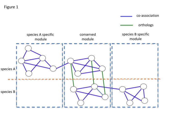
Figure 1 co-association orthologs species B specific module conserved module species A specific module species A species B
Figure 2 Set initial temperature T(0) Orthologous pairs between species randomly assign labels (1,2,..,q) to nodes simulated annealing to optimize H Co-association network of species A Cost function H system evolves (labels flip) according to H Co-association network of species B T(k+1) = T(k) flipping rate is low? Extendable to more species Potts Clustering at most q modules labeled by 1 to q Input High-confidence modules based on multiple runs A set of cross-species modules, with different number of shared orthologs Output A-specific module B-specific module conserved module
Figure 3A worm and fly genes Sharing of GO terms 218 231 worm (20377) 117 Conserved module 16 14 fly (13623) worm specific module fly specific module co-appear frequency
Figure 3B GO terms of a conserved module 4
Figure 4 5
Figure 5 A B 1 0.04 1 optimal k the highest modularity 0.9 0.035 0.8 Fraction of Gold Standard covered in modules modularity of the GO reference network 0.03 Modularity of individual networks 0.7 0.6 0.025 fly 0.5 0.5 0.02 0.4 0.3 0.015 worm 0.2 0.01 0.1 0 0.005 50 0 0.5 1 1.5 2 coupling constant k 2.5 3 3.5 4 4.5 5 0 0.5 1 1.5 2 2.5 3 3.5 4 4.5 coupling constant k
Figure 6 7
Figure 7 8
Figure S1 Flipping rate the number of sweep
Figure S2 10
Figure S3 11
Figure S4 average number of common TFs (normalized) worm modules fly modules
Figure S5 Number of modules by unweighted clustering Number of modules by weighted clustering Number of worm genes Number of fly genes worm 67 22 1 68 20 43 1 31 8 25 1 17 .. 5 23 1 6 fly 20 8 1 23 18 12 1 16 17 17 1 2 8 17 1 22 17 2 7 17 13 10 1 4
Figure S6 1 0.95 Fraction of metagenes recovered by Isorank 0.9 0.85 0.8 0.75 0.7 0.65 0.6 0.1 0.2 0.3 0.4 0.5 a 0.6 0.7 0.8 0.9
Figure S8 1 worm (5769) co-appearance frequency fly (5507) 0
Figure S9 Enrichment -log(P-value)