Chapter 4 Physics-based Prognostics

C
h
a
p
t
e
r
4
P
h
y
s
i
c
s
-
b
a
s
e
d
P
r
o
g
n
o
s
t
i
c
s
1. Introduction to Physics-based Prognostics
•
Physics-based prognostics
: there exists a physical model that
describes the evolution of damage or degradation (degradation model)
•
Key issues: how to improve the accuracy of degradation model and
how to incorporate uncertainty in the future
•
Sources of uncertainty
–
Uncertainty in model parameters
–
Uncertainty in loading conditions
–
Error in the model form
•
Decision-making process of prognostics should include these sources
of uncertainty and should be based on conservative estimate of
damage degradation
P
a
r
a
m
e
t
e
r
E
s
t
i
m
a
t
i
o
n
i
n
P
r
o
g
n
o
s
t
i
c
s
I
l
l
u
s
t
r
a
t
i
o
n
o
f
P
h
y
s
i
c
s
-
b
a
s
e
d
P
r
o
g
n
o
s
t
i
c
s
U
n
c
e
r
t
a
i
n
t
y
i
n
M
o
d
e
l
P
a
r
a
m
e
t
e
r
s
N=0:100:4000;sig=70;a0=0.001; m=3.6:0.1:4.2; C=5E-10; figure; hold on;
for i=1:7
a(i,:)=(N.*C*(1-m(i)/2)*(sig*sqrt(pi))^m(i)+a0^(1-m(i)/2)).^(2/(2-m(i)));
plot(N,a(i,:));
end
E
f
f
e
c
t
o
f
M
o
d
e
l
P
a
r
a
m
e
t
e
r
U
n
c
e
r
t
a
i
n
t
y
•
uncertainty in model parameters is mostly from epistemic uncertainty
•
The fundamental concept of physics-based prognostics is to use
measurement data to reduce the uncertainty in model parameters
–
measurement data can be used to reduce the uncertainty in degradation
model parameters using the Bayesian framework
–
most physics-based prognostics methods have their foundation on Bayesian
inference
•
Once model parameters are identified, the future behavior of
degradation can be predicted by propagating the model to the future
–
substitute the identified parameters to the degradation model with future time
and loadings
–
the RUL is predicted by propagating the degradation state until it reaches a
threshold
E
p
i
s
t
e
m
i
c
U
n
c
e
r
t
a
i
n
t
y
i
n
M
o
d
e
l
P
a
r
a
m
e
t
e
r
s
•
Physics-based prognostics methods are based on parameter estimation
algorithms
•
Nonlinear least squares (NLS): nonlinear version of least squares method
•
Bayesian method (BM): Overall Bayesian inference
•
Kalman filter (KF): exact posterior distribution in the case of a linear
system with Gaussian noise
•
Extended/unscented Kalman filter: for nonlinear systems
•
Particle filter (PF): represent the posterior distribution using particles
P
h
y
s
i
c
s
-
b
a
s
e
d
P
r
o
g
n
o
s
t
i
c
s
M
e
t
h
o
d
s
D
e
m
o
n
s
t
r
a
t
i
o
n
P
r
o
b
l
e
m
:
B
a
t
t
e
r
y
D
e
g
r
a
d
a
t
i
o
n
D
e
g
r
a
d
a
t
i
o
n
D
a
t
a
2. Nonlinear Least Squares (NLS)
•
We used least squares method in Chapter 2
–
Regression: when unknown model parameters are linear in the model
•
Nonlinear least squares (NLS)
–
When the model parameters are nonlinear relationship in the model
•
How do you know a model is nonlinear?
–
Derivatives depends on parameters
•
Ex) Battery degradation
•
NLS finds the best parameters using the weighted sum of square errors
N
o
n
l
i
n
e
a
r
L
e
a
s
t
S
q
u
a
r
e
s
M
e
t
h
o
d
N
o
n
l
i
n
e
a
r
L
e
a
s
t
S
q
u
a
r
e
s
M
e
t
h
o
d
c
o
n
t
.
U
n
c
e
r
t
a
i
n
t
y
i
n
N
L
S
N
L
S
:
M
a
t
l
a
b
c
o
d
e
f
o
r
N
o
n
l
i
n
e
a
r
L
e
a
s
t
S
q
u
a
r
e
s
function
[thetaHat,rul]=NLS(theta0)
clear
global
;
global
DegraUnit TimeUnit
...
time y thres ParamName thetaTrue signiLevel ns ny nt np
%=== PROBLEM DEFINITION 1 (Required Variables) ==============
WorkName=
' '
;
% work results are saved by WorkName
DegraUnit=
' '
;
% degradation unit
TimeUnit=
' '
;
% time unit (Cycles, Weeks, etc.)
time=[ ]';
% time at both measurement and prediction
y=[ ]';
%[nyx1]: measured data
thres= ;
% threshold (critical value)
ParamName=[ ];
%[npx1]: parameters' name to be estimated
thetaTrue=[ ];
%[npx1]: true values of parameters
signiLevel= ;
% significance level for C.I. and P.I.
ns= ;
% number of particles/samples
N
L
S
M
a
t
l
a
b
C
o
d
e
c
o
n
t
.
%============================================================
% % % PROGNOSIS using NLS
ny=length(y); nt=ny;
np=size(ParamName,1);
%% Deterministic Estimation
Optio=optimset(
'algorithm'
,{'levenberg-marquardt'
,0.01});
[thetaH,~,resid,~,~,~,J]=lsqnonlin(@FUNC,theta0,[],[],Optio);
sse=resid'*resid;
%% Distribution of Theta
dof=ny-np+1;
sigmaH=sqrt(sse/dof);
% Estimated std of data
W=eye(ny)*1/sigmaH^2; thetaCov=inv(J'*W*J);
sigTheta=sqrt(diag(thetaCov));
% Estimated std of Theta
mvt=mvtrnd(thetaCov,dof,ns)';
% Generate t-dist
thetaHat=repmat(thetaH,1,ns)+mvt.*repmat(sigTheta,1,ns);
thetaHat(np,:)=sigmaH*ones(1,ns);
%% Final Sampling Results
for
k=1:length(time(ny:end));
%% Degradation Prediction
zHat(k,:)=MODEL(thetaHat,time(ny-1+k));
degraPredi(k,:)=zHat(k,:)+trnd(dof,1,ns)*sigmaH;
end
;
N
L
S
M
a
t
l
a
b
C
o
d
e
c
o
n
t
.
% % % POST-PROCESSING
degraTrue=[];
%% True Degradation
if
~isempty(thetaTrue); degraTrue=MODEL(thetaTrue,time);
end
rul=POST(thetaHat,degraPredi,degraTrue);
%% RUL & Result Disp
Name=[WorkName
' at '
num2str(time(ny))
'.mat'
]; save(Name);
end
function
objec=FUNC(theta)
global
time y ny
z=MODEL(theta,time(1:ny));
objec=(y-z);
end
function
z=MODEL(theta,t)
global
ParamName np
for
j=1:np-1; eval([ParamName(j,:)
'=theta(j,:);'
]);
end
%===== PROBLEM DEFINITION 2 (model equation) ===============
%===========================================================
end
•
Matlab code NLS is a template
–
Users can define their own degradation model with unknown model
parameters
1.
Problem definition for user-specific applications
–
Variable definition
–
Model definition
2.
Prognostics using NLS
3.
Post-processing for displaying results
N
L
S
C
o
d
e
E
x
p
l
a
n
a
t
i
o
n
P
r
o
b
l
e
m
D
e
f
i
n
i
t
i
o
n
s
(
l
i
n
e
s
5
-
1
4
,
4
8
)
•
Lines 5-14
•
Line 48
P
r
o
b
l
e
m
D
e
f
i
n
i
t
i
o
n
f
o
r
B
a
t
t
e
r
y
D
e
g
r
a
d
a
t
i
o
n
WorkName='Battery_NLS';
DegraUnit='C/1 Capacity';
TimeUnit='Cycles';
time=[0:5:200]';
y=[1.00 0.99 0.99 0.94 0.95 0.94 0.91 0.91 0.87 0.86]';
thres=0.7;
ParamName=['b'; 's'];
thetaTrue=[0.003; 0.02];
signiLevel=5;
ns=5e3;
z=exp(-b.*t);
•
Use LM algorithm with more dominant use of Gauss-Newton update
•
Minimize FUNC starting from theta0 using
lsqnonlin
P
r
o
g
n
o
s
t
i
c
s
U
s
i
n
g
N
L
S
(
l
i
n
e
s
1
7
-
3
2
)
Optio=optimset(
'algorithm'
,{'levenberg-marquardt'
,0.01});
[thetaH,~,resid,~,~,~,J]=lsqnonlin(@FUNC,theta0,[],[],Optio);
function
objec=FUNC(theta)
global
time y ny
z=MODEL(theta,time(1:ny));
objec=(y-z);
end
function
z=MODEL(theta,t)
global
ParamName np
for
j=1:np-1; eval([ParamName(j,:)
'=theta(j,:);'
]);
end
%===== PROBLEM DEFINITION 2 (model equation) ===============
%===========================================================
end
P
r
o
g
n
o
s
t
i
c
s
U
s
i
n
g
N
L
S
W=eye(ny)*1/sigmaH^2; thetaCov=inv(J'*W*J);
sigTheta=sqrt(diag(thetaCov));
% Estimated std of Theta
sse=resid'*resid;
%% Distribution of Theta
dof=ny-np+1;
sigmaH=sqrt(sse/dof);
% Estimated std of data
mvt=mvtrnd(thetaCov,dof,ns)';
% Generate t-dist
thetaHat=repmat(thetaH,1,ns)+mvt.*repmat(sigTheta,1,ns);
thetaHat(np,:)=sigmaH*ones(1,ns);
%% Final Sampling Results
for
k=1:length(time(ny:end));
%% Degradation Prediction
zHat(k,:)=MODEL(thetaHat,time(ny-1+k));
degraPredi(k,:)=zHat(k,:)+trnd(dof,1,ns)*sigmaH;
end
;
•
Plots of model parameters and RUL using Matlab code POST
•
Save database to the disk
•
How to use NLS
–
LM algorithm in lsqnonlin finds a local optimum (depending on initial)
P
o
s
t
-
p
r
o
c
e
s
s
i
n
g
(
l
i
n
e
s
3
4
-
3
7
)
%%% POST-PROCESSING
degraTrue=[];
%% True Degradation
if
~isempty(thetaTrue); degraTrue=MODEL(thetaTrue,time);
end
rul=POST(thetaHat,degraPredi,degraTrue);
%% RUL & Result Disp
Name=[WorkName
' at '
num2str(time(ny))
'.mat'
]; save(Name);
[thetaHat,rul]=NLS(0.01);
M
a
t
l
a
b
C
o
d
e
P
O
S
T
function
rul=POST(thetaHat,degraPredi,degraTrue)
for
j=1:np; subplot(1,np,j);
[frq,val]=hist(thetaHat(j,:),30);
bar(val,frq/ns/(val(2)-val(1)));
xlabel(ParamName(j,:));
end
;
degraPI=prctile(degraPredi',perceValue)';
f1(1,:)=plot(time(1:ny),y(:,1),
'.k'
); hold
on
;
f1(2,:)=plot(time(ny:end),degraPI(:,1),
'--r'
);
f1(3:4,:)=plot(time(ny:end),degraPI(:,2:3),
':r'
);
f2=plot([0 time(end)],[thres thres],
'g'
);
•
RUL calculation
–
coeff =1 (increasing) or -1 (decreasing) degradation
–
loca: location when degradation reaches the threshold
–
i0: number of samples that did not reach the threshold (never failed)
M
a
t
l
a
b
C
o
d
e
P
O
S
T
i0=0;
%% RUL Prediction
if
y(nt(1))-y(1)<0; coeff=-1;
else
coeff=1;
end
;
for
i=1:ns;
loca=find(degraPredi(:,i)*coeff>=thres*coeff,1);
if
isempty(loca); i0=i0+1;
disp([num2str(i)
'th not reaching thres'
]);
elseif
loca==1; rul(i-i0)=0;
else
rul(i-i0)=
...
interp1([degraPredi(loca,i) degraPredi(loca-1,i)],
...
[time(ny-1+loca) time(ny-2+loca)],thres)-time(ny);
end
end
;
rulPrct=prctile(rul,perceValue);
•
Plotting the histogram of RUL
M
a
t
l
a
b
C
o
d
e
P
O
S
T
c
o
n
t
.
figure(3);
%% RUL Results Display
[frq,val]=hist(rul,30);
bar(val,frq/ns/(val(2)-val(1))); hold
on
;
xlabel([
'RUL'
' ('TimeUnit
')'
]);
titleName=[
'at '
num2str(time(ny))
' '
TimeUnit];
title(titleName)
fprintf([
'\n Percentiles of RUL at %g '
TimeUnit], time(ny))
fprintf(
'\n %gth: %g, 50th (median): %g, %gth: %g \n'
,
...
perceValue(2),rulPrct(2),rulPrct(1),perceValue(3),rulPrct(3))
3. Bayesian Method (BM)
•
In terms of Chapter 3, BM corresponds to overall Bayesian method
–
All training data (up to the current time) are used together to build the
likelihood function
–
The posterior distribution is obtained by multiplying the likelihood function
with the prior distribution
•
For conjugate distribution, it is possible to generate samples from
standard distributions
•
For single parameter estimation, the inverse CDF method can be used
to generate samples
•
For general cases, Markov-chain Monte-Carly (MCMC) method will be
used to generate samples
•
Using generated samples of model parameters, samples of RUL can be
generated
B
a
y
e
s
i
a
n
M
e
t
h
o
d
(
B
M
)
E
x
)
M
C
M
C
M
e
t
h
o
d
:
O
n
e
P
a
r
a
m
e
t
e
r
para0=5; weigh=5;
for i=1:5000
u=rand;
para1=unifrnd(para0-weigh, para0+weigh);
pdf1=normpdf(para1,5,2.9);
pdf0=normpdf(para0,5,2.9);
Q=min(1, pdf1/pdf0);
u=rand;
if u<Q; sampl(:,i)=para1; else sampl(:,i)=para0; end
para0=sampl(:,i);
end
plot(sampl); xlabel('Iteration (samples)'); ylabel('A')figure; [frq,val]=hist(sampl,30);
bar(val,frq/5000/(val(2)-val(1))); hold on;
a=-10:0.1:20; plot(a,normpdf(a,5,2.9),'k')
xlabel('A'); legend('Sampling','Exact')•
The quality of proposal distribution can be assessed using the trace of
samples
•
Ex) para0=0.5, weigh=0.5
•
Trace does not show fluctuation with respect to the mean
•
The histogram does not agree with the analytical PDF
E
x
)
M
C
M
C
M
e
t
h
o
d
:
O
n
e
P
a
r
a
m
e
t
e
r
c
o
n
t
.
E
x
)
M
u
l
t
i
d
i
m
e
n
s
i
o
n
a
l
C
o
r
r
e
l
a
t
e
d
S
a
m
p
l
i
n
g
para0=[0; 1]; weigh=[0.05; 0.05]; s=2.9;
t = [0 1 2 3 4];
y=[6.99 2.28 1.91 11.94 14.60];
f0=5+para0(1)*t.^2+para0(2)*t.^3;
pdf0=(s*sqrt(2*pi))^-5*exp(-(f0-y)*(f0-y)'/(2*s^2));
para1=unifrnd(para0-weigh, para0+weigh);
f1=5+para1(1)*t.^2+para1(2)*t.^3;
pdf1=(s*sqrt(2*pi))^-5*exp(-(f1-y)*(f1-y)'/(2*s^2));
•
Due to a wrong initial point, first 200 samples are disregarded (burn-in)
•
Sample trace show that the weight is too small
•
para0=[0; 0], weigh=[0.3; 0.3]
,
E
x
)
M
u
l
t
i
d
i
m
e
n
s
i
o
n
a
l
C
o
r
r
e
l
a
t
e
d
S
a
m
p
l
i
n
g
c
o
n
t
.
•
Problem definition
B
a
y
e
s
i
a
n
M
e
t
h
o
d
M
a
t
l
a
b
C
o
d
e
(
B
M
)
function
[thetaHat,rul]=BM(para0,weigh)
clear
global
;
global
DegraUnit initDisPar TimeUnit
...
time y thres ParamName thetaTrue signiLevel ns ny nt np
%=== PROBLEM DEFINITION 1 (Required Variables) ==============
WorkName=
' '
;
% work results are saved by WorkName
DegraUnit=
' '
;
% degradation unit
TimeUnit=
' '
;
% time unit (Cycles, Weeks, etc.)
time=[ ]';
% time at both measurement and prediction
y=[ ]';
%[nyx1]: measured data
thres= ;
% threshold (critical value)
ParamName=[ ];
%[npx1]: parameters' name to be estimated
initDisPar=[ ];
%[npx2]: prob. parameters of init./prior dist
thetaTrue=[ ];
%[npx1]: true values of parameters
signiLevel= ;
% significance level for C.I. and P.I.
ns= ;
% number of particles/samples
burnIn= ;
% ratio for burn-in
B
M
M
a
t
l
a
b
C
o
d
e
c
o
n
t
.
%============================================================
% % % PROGNOSIS using BM with MCMC
ny=length(y); nt=ny;
np=size(ParamName,1);
sampl(:,1)=para0;
%% Initial Samples
[~,jPdf0]=MODEL(para0,time(1:ny));
%% Initial (joint) PDF
for
i=2:ns/(1-burnIn);
%% MCMC Process
% proposal distribution (uniform)
para1(:,1)=unifrnd(para0-weigh,para0+weigh);
% (joint) PDF at new samples
[~,jPdf1]=MODEL(para1,time(1:ny));
% acceptance/rejection criterion
if
rand<min(1,jPdf1/jPdf0)
para0=para1; jPdf0=jPdf1;
end
;
sampl(:,i)=para0;
end
;
nBurn=ns/(1-burnIn)-ns;
%% Sampling Trace
figure(4);
for
j=1:np;subplot(np,1,j);plot(sampl(j,:));hold
on
plot([nBurn nBurn],[min(sampl(j,:)) max(sampl(j,:))],
'r'
);
end
thetaHat=sampl(:,nBurn+1:end);
%% Final Sampling Results
for
k=1:length(time(ny:end));
%% Degradation Prediction
[zHat(k,:),~]=MODEL(thetaHat,time(ny-1+k));
degraPredi(k,:)=normrnd(zHat(k,:),thetaHat(end,:));
end
;
B
M
M
a
t
l
a
b
C
o
d
e
c
o
n
t
.
% % % POST-PROCESSING
degraTrue=[];
%% True Degradation
if
~isempty(thetaTrue); degraTrue=MODEL(thetaTrue,time);
end
rul=POST(thetaHat,degraPredi,degraTrue);
%% RUL & Result Disp
Name=[WorkName
' at '
num2str(time(ny))
'.mat'
]; save(Name);
end
function
[z,poste]=MODEL(param,t)
global
y ParamName initDisPar ny np
for
j=1:np; eval([ParamName(j,:)
'=param(j,:);'
]);
end
%===== PROBLEM DEFINITION 2 (model equation) ===============
%===========================================================
if
length(y)~=length(t); poste=[];
else
prior=
...
%% Prior
prod(unifpdf(param,initDisPar(:,1),initDisPar(:,2)));
likel=(1./(sqrt(2.*pi).*s)).^ny.*
...
%% Likelihood
exp(-0.5./s.^2.*(y-z)'*(y-z));
poste=likel.*prior;
%% Posterior
end
end
•
Normal likelihood
•
Prior distribution:
•
Problem definition (lines 5-16, 52)
–
initDisPar: initial distribution parameters
–
burnIn=0.2: initial 20% of samples will be discarded
•
All other problem definitions are the same as NLS
B
M
I
m
p
l
e
m
e
n
t
a
t
i
o
n
f
o
r
B
a
t
t
e
r
y
P
r
o
g
n
o
s
t
i
c
s
initDisPar=[0 0.02; 1e-5 0.1];
burnIn=0.2;
•
Calling BM:
–
Initial parameters param0 =
[0.01 0.05]’
–
Weight of proposal distribution =
[0.0005 0.01]’
–
thetaHat: samples of estimated model parameters
–
rul: samples of RUL
•
Two usages of MODEL
–
MODEL returns degradation prediction z, and posterior PDF
–
During model parameter estimation, posterior PDF poste is calculated using
ny data
–
During prognostics, MODEL is used to generate future degradation samples
with future time
B
M
I
m
p
l
e
m
e
n
t
a
t
i
o
n
f
o
r
B
a
t
t
e
r
y
P
r
o
g
n
o
s
t
i
c
s
c
o
n
t
.
[thetaHat,rul]=BM([0.01 0.05]',[0.0005 0.01]');
function
[z,poste]=MODEL(param,t)
O
v
e
r
a
l
l
B
M
P
o
s
t
e
r
i
o
r
P
D
F
if
length(y)~=length(t); poste=[];
else
prior=
...
%% Prior
prod(unifpdf(param,initDisPar(:,1),initDisPar(:,2)));
likel=(1./(sqrt(2.*pi).*s)).^ny.*
...
%% Likelihood
exp(-0.5./s.^2.*(y-z)'*(y-z));
poste=likel.*prior;
%% Posterior
end
•
Parameter estimation = generating samples from posterior distribution
–
Using MCMC sampling
P
r
o
g
n
o
s
t
i
c
s
u
s
i
n
g
B
M
sampl(:,1)=para0;
%% Initial Samples
[~,jPdf0]=MODEL(para0,time(1:ny));
%% Initial (joint) PDF
for
i=2:ns/(1-burnIn);
%% MCMC Process
% proposal distribution (uniform)
para1(:,1)=unifrnd(para0-weigh,para0+weigh);
% (joint) PDF at new samples
[~,jPdf1]=MODEL(para1,time(1:ny));
% acceptance/rejection criterion
if
rand<min(1,jPdf1/jPdf0)
para0=para1; jPdf0=jPdf1;
end
;
sampl(:,i)=para0;
end
;
•
Remove the first nBurn samples
–
Remaining number of samples = ns
S
a
m
p
l
i
n
g
T
r
a
c
e
nBurn=ns/(1-burnIn)-ns;
%% Sampling Trace
figure(4);
for
j=1:np;subplot(np,1,j);plot(sampl(j,:));hold
on
plot([nBurn nBurn],[min(sampl(j,:)) max(sampl(j,:))],
'r'
);
end
•
Basically the same with NLS
–
Use POST with samples of parameters and degradations
P
o
s
t
-
p
r
o
c
e
s
s
i
n
g
(
l
i
n
e
s
4
3
-
4
6
)
Percentiles of RUL at 45 Cycles
5th: 54.3859,
50th (median): 68.3619,
95th: 82.8892
4. Particle Filter (PF)
•
the most popular method in the physics-based prognostics
–
fundamental concept is the same as the recursive Bayesian update
•
the prior and posterior PDF of parameters are represented by particles
(samples)
•
the posterior at the previous step is used as the prior at the current
step, and the parameters are updated by multiplying it with the
likelihood from the new measurement
•
also known as the sequential Monte Carlo method
P
a
r
t
i
c
l
e
F
i
l
t
e
r
R
e
v
i
e
w
o
f
I
m
p
o
r
t
a
n
c
e
S
a
m
p
l
i
n
g
(
I
S
)
•
PF can be considered as a sequential importance sampling method
–
weights are continuously updated whenever a new observation is available
•
Degeneracy phenomenon
–
happens when weights are updated with the same initial samples
–
decreases the accuracy in the posterior distribution with a large variance
•
sequential importance resampling (SIR)
–
Small weight particles are removed
–
High weight particles are duplicated
S
e
q
u
e
n
t
i
a
l
I
S
G
e
n
e
r
a
l
P
r
o
c
e
s
s
o
f
P
F
•
Rewrite the battery degradation model in terms of PF process
•
Ratio
•
PF form:
A
p
p
l
i
c
a
t
i
o
n
t
o
B
a
t
t
e
r
y
D
e
g
r
a
d
a
t
i
o
n
S
I
R
P
r
o
c
e
s
s
S
I
R
P
r
o
c
e
s
s
:
P
r
e
d
i
c
t
i
o
n
S
I
R
P
r
o
c
e
s
s
:
U
p
d
a
t
e
S
I
R
P
r
o
c
e
s
s
:
U
p
d
a
t
e
c
o
n
t
.
S
I
R
P
r
o
c
e
s
s
:
R
e
s
a
m
p
l
i
n
g
S
I
R
P
r
o
c
e
s
s
:
R
e
s
a
m
p
l
i
n
g
c
o
n
t
.
E
x
)
P
F
o
f
B
a
t
t
e
r
y
D
e
g
r
a
d
a
t
i
o
n
w
i
t
h
1
0
S
a
m
p
l
e
s
k=1; ns=10;
b(k,:)=unifrnd(0,0.005,ns,1);
z(k,:)=unifrnd(0.9,1.1,ns,1);
figure; subplot(1,2,1);
plot(b(k,:),zeros(1,ns),'ok'); xlabel('b (parameter)')subplot(1,2,2);
plot(z(k,:),zeros(1,ns),'ok'); xlabel('z (degradation)')E
x
)
P
F
o
f
B
a
t
t
e
r
y
D
e
g
r
a
d
a
t
i
o
n
w
i
t
h
1
0
S
a
m
p
l
e
s
k=2; dt=5;
b(k,:)=b(k-1,:);
z(k,:)=exp(-b(k,:).*dt).*z(k-1,:);
% for figure plot, use the same code given in k=1
E
x
)
P
F
o
f
B
a
t
t
e
r
y
D
e
g
r
a
d
a
t
i
o
n
w
i
t
h
1
0
S
a
m
p
l
e
s
likel=normpdf(y(k,:),z(k,:),0.02);
weigh=round(likel/sum(likel)*ns);
figure; subplot(1,2,1); stem(b(k,:),weigh,'r');
xlabel('b (parameter)'); ylabel('Weight')subplot(1,2,2); stem(z(k,:),weigh,'r');
xlabel('z (degradation)'); ylabel('Weight')E
x
)
P
F
o
f
B
a
t
t
e
r
y
D
e
g
r
a
d
a
t
i
o
n
w
i
t
h
1
0
S
a
m
p
l
e
s
sampl=[b(k,:); z(k,:)];
loca=find(weigh>0); ns0=1;
for i=1:length(loca);
ns1=sum(weigh(loca(1:i)));
b(k,ns0:ns1)=sampl(1,loca(i))*ones(1,weigh(loca(i)));
z(k,ns0:ns1)=sampl(2,loca(i))*ones(1,weigh(loca(i)));
ns0=ns1+1;
end
Several samples are overlapped:
particle depletion
E
x
)
P
F
o
f
B
a
t
t
e
r
y
D
e
g
r
a
d
a
t
i
o
n
w
i
t
h
1
0
S
a
m
p
l
e
s
E
x
)
P
F
o
f
B
a
t
t
e
r
y
D
e
g
r
a
d
a
t
i
o
n
w
i
t
h
1
0
S
a
m
p
l
e
s
P
a
r
t
i
c
l
e
F
i
l
t
e
r
(
P
F
)
M
a
t
l
a
b
C
o
d
e
function
[thetaHat,rul]=PF
clear
global
;
global
DegraUnit initDisPar TimeUnit
...
time y thres ParamName thetaTrue signiLevel ns ny nt np
%=== PROBLEM DEFINITION 1 (Required Variables) ==============
WorkName=
' '
;
% work results are saved by WorkName
DegraUnit=
' '
;
% degradation unit
TimeUnit=
' '
;
% time unit (Cycles, Weeks, etc.)
time=[ ]';
% time at both measurement and prediction
dt= ;
% time interval for degradation propagation
y=[ ]';
%[nyx1]: measured data
thres= ;
% threshold (critical value)
ParamName=[ ];
%[npx1]: parameters' name to be estimated
initDisPar=[ ];
%[npx2]: prob. parameters of init./prior dist
thetaTrue=[ ];
%[npx1]: true values of parameters
signiLevel= ;
% significance level for C.I. and P.I.
ns= ;
% number of particles/samples
P
F
M
a
t
l
a
b
C
o
d
e
c
o
n
t
.
% % % PROGNOSIS using PF
ny=length(y); nt=ny;
np=size(ParamName,1);
for
j=1:np;
%% Initial Distribution
param(j,:,1)=unifrnd(initDisPar(j,1),initDisPar(j,2),1,ns);
end
;
for
k=2:length(time);
%% Update Process or Prognosis
paramPredi=param(:,:,k-1);
% step1. prediction (prior)
nk=(time(k)-time(k-1))/dt;
for
k0=1:nk; paramPredi(np,:)=MODEL(paramPredi,dt);
end
if
k<=ny
% (Update Process)
% step2. update (likelihood)
likel=normpdf(y(k),paramPredi(np,:),paramPredi(np-1,:));
cdf=cumsum(likel)./sum(likel);
% step3. resampling
for
i=1:ns;
u=rand;
loca=find(cdf>=u,1); param(:,i,k)=paramPredi(:,loca);
end
;
else
% (Prognosis)
param(:,:,k)=paramPredi;
end
end
thetaHat=param(1:np-1,:,ny);
%% Final Sampling Results
paramRearr=permute(param,[3 2 1]);
%% Degradation Prediction
zHat=paramRearr(:,:,np);
degraPredi=normrnd(zHat(ny:end,:),paramRearr(ny:end,:,np-1));
P
F
M
a
t
l
a
b
C
o
d
e
c
o
n
t
.
% % % POST-PROCESSING
degraTrue=[];
%% True Degradation
if
~isempty(thetaTrue); k=1;
degraTrue0(1)=thetaTrue(np); degraTrue(1)=thetaTrue(np);
for
k0=2:max(time)/dt+1;
degraTrue0(k0,1)=
...
MODEL([thetaTrue(1:np-1); degraTrue0(k0-1)],dt);
loca=find((k0-1)*dt==time,1);
if
~isempty(loca); k=k+1; degraTrue(k)=degraTrue0(k0);
end
end
end
rul=POST(thetaHat,degraPredi,degraTrue);
%% RUL & Result Disp
Name=[WorkName
' at '
num2str(time(ny))
'.mat'
]; save(Name);
end
function
z1=MODEL(param,dt)
global
ParamName np
for
j=1:np; eval([ParamName(j,:)
'=param(j,:);'
]);
end
%===== PROBLEM DEFINITION 2 (model equation) ===============
%===========================================================
end
M
a
t
l
a
b
I
m
p
l
e
m
e
n
t
a
t
i
o
n
f
o
r
B
a
t
t
e
r
y
P
r
o
g
n
o
s
t
i
c
s
dt=5;
ParamName=['b'; 's'; 'z'];
initDisPar=[0 0.02; 1e-5 0.1; 1 1];
thetaTrue=[0.003; 0.02; 1];
z1=exp(-b.*dt).*z;
M
a
t
l
a
b
I
m
p
l
e
m
e
n
t
a
t
i
o
n
f
o
r
B
a
t
t
e
r
y
P
r
o
g
n
o
s
t
i
c
s
[thetaHat,rul]=PF;
for
j=1:np;
%% Initial Distribution
param(j,:,1)=unifrnd(initDisPar(j,1),initDisPar(j,2),1,ns);
end
;
M
a
t
l
a
b
I
m
p
l
e
m
e
n
t
a
t
i
o
n
f
o
r
B
a
t
t
e
r
y
P
r
o
g
n
o
s
t
i
c
s
% step1. prediction (prior)
paramPredi=param(:,:,k-1);
nk=(time(k)-time(k-1))/dt;
for
k0=1:nk; paramPredi(np,:)=MODEL(paramPredi,dt);
end
if
k<=ny
% (Update Process)
% step2. update (likelihood)
likel=normpdf(y(k),paramPredi(np,:),paramPredi(np-1,:));
M
a
t
l
a
b
I
m
p
l
e
m
e
n
t
a
t
i
o
n
f
o
r
B
a
t
t
e
r
y
P
r
o
g
n
o
s
t
i
c
s
% step3. resampling
cdf=cumsum(likel)./sum(likel);
for
i=1:ns;
u=rand;
loca=find(cdf>=u,1);
param(:,i,k)=paramPredi(:,loca);
end
;
else
% (Prognosis)
param(:,:,k)=paramPredi;
end
•
Post-processing
–
Basically identical to NLS and BM
–
Since degradation is a part of param, rearrange arrayes
M
a
t
l
a
b
I
m
p
l
e
m
e
n
t
a
t
i
o
n
f
o
r
B
a
t
t
e
r
y
P
r
o
g
n
o
s
t
i
c
s
thetaHat=param(1:np-1,:,ny);
%% Final Sampling Results
paramRearr=permute(param,[3 2 1]);
%% Degradation Prediction
zHat=paramRearr(:,:,np);
degraPredi=normrnd(zHat(ny:end,:),paramRearr(ny:end,:,np-1));
5. Practical Application of Physics-based
Prognostics
C
r
a
c
k
G
r
o
w
t
h
M
o
d
e
l
D
e
f
i
n
i
t
i
o
n
C
r
a
c
k
G
r
o
w
t
h
M
o
d
e
l
D
e
f
i
n
i
t
i
o
n
•
In order to study the effect of different distribution type, we assume
likelihood is from a lognormal distribution
–
This means that random measurement noise is lognormally distributed
–
Standard deviation:
–
Mean:
•
Prior distribution
L
i
k
e
l
i
h
o
o
d
a
n
d
P
r
i
o
r
D
i
s
t
r
i
b
u
t
i
o
n
M
o
d
i
f
y
i
n
g
N
L
S
M
a
t
l
a
b
C
o
d
e
WorkName='Crack_NLS';
DegraUnit='Crack size (m)';
TimeUnit='Cycles';
time=[0:100:3500]';
y=[0.0100 0.0109 0.0101 0.0107 0.0110 0.0123 0.0099 0.0113
...
0.0132 0.0138 0.0148 0.0156 0.0155 0.0141 0.0169 0.0168]';
thres=0.05;
ParamName=['m'; 'C'; 's'];
thetaTrue=[3.8; log(1.5e-10); 0.001];
signiLevel=5;
ns=5e3;
M
o
d
i
f
y
i
n
g
N
L
S
M
a
t
l
a
b
C
o
d
e
c
o
n
t
.
a0=0.01; dsig=75;
z=(t.*exp(C).*(1-m./2).*(dsig*sqrt(pi)).^m ...
+a0.^(1-m./2)).^(2./(2-m));
loca=imag(z)~=0; z(loca)=1;
•
Likelihood
–
Likelihood is unnecessary for NLS, but it is used to predict degradation
•
Calling NLS
M
o
d
i
f
y
i
n
g
N
L
S
M
a
t
l
a
b
C
o
d
e
c
o
n
t
.
mu=zHat(k,:);
C=chi2rnd(ny-1,1,ns);
s=sqrt((ny-1)*thetaHat(np,:).^2./C);
zeta=sqrt(log(1+(s./mu).^2)); eta=log(mu)-0.5*zeta.^2;
degraPredi(k,:)=lognrnd(eta,zeta);
[thetaHat,rul]=NLS([4; -23]);
M
o
d
i
f
y
i
n
g
B
M
M
a
t
l
a
b
C
o
d
e
WorkName='Crack_BM';
initDisPar=[4.0 0.2; -23 1.1; 0.001 1e-5];
burnIn=0.2;
prior=prod(normpdf(param,initDisPar(:,1),initDisPar(:,2)));
likel=1;
for k=1:ny;
zeta=sqrt(log(1+(s./z(k)).^2)); eta=log(z(k))-0.5*zeta.^2;
likel=lognpdf(y(k),eta,zeta).*likel;
end
[thetaHat]=BM([4 -23 0.001]',[0.1 0.2 0]');
•
Problem definition
–
PF includes state ‘a’ as the last parameter
•
Model definition
M
o
d
i
f
y
i
n
g
P
F
M
a
t
l
a
b
C
o
d
e
WorkName='Crack_PF';
dt=20;
ParamName=['m'; 'C'; 's'; 'a'];
initDisPar=[4.0 0.2; -23 1.1; 0.001 0; 0.01 0];
thetaTrue=[3.8;log(1.5e-10); 0.001; 0.01];
dsig=75;
z1=exp(C).*(dsig.*sqrt(pi*a)).^m.*dt+a;
•
Predicting degradation (logarithmic distribution)
•
Initial distribution
•
Likelihood (weight)
•
Calling PF
M
o
d
i
f
y
i
n
g
P
F
M
a
t
l
a
b
C
o
d
e
c
o
n
t
.
mu=zHat(ny:end,:); s=paramRearr(ny:end,:,np-1);
zeta=sqrt(log(1+(s./mu).^2)); eta=log(mu)-0.5*zeta.^2;
degraPredi=lognrnd(eta,zeta);
param(j,:,1)=normrnd(initDisPar(j,1),initDisPar(j,2),1,ns);
mu=paramPredi(np,:); s=paramPredi(np-1,:);
zeta=sqrt(log(1+(s./mu).^2)); eta=log(mu)-0.5*zeta.^2;
likel=lognpdf(y(k),eta,zeta);
[thetaHat,rul]=PF;
•
Correlation plot
–
A large uncertainty in the results from NLS compared to the others (because
no prior information is employed)
–
Large uncertainty in parameters leads to large uncertainty in degradation
prediction
–
PF is still not showing smooth distribution of particles
C
o
m
p
a
r
i
s
o
n
o
f
R
e
s
u
l
t
s
plot(thetaHat(1,:),thetaHat(2,:),'.')
.
C
o
m
p
a
r
i
s
o
n
o
f
R
e
s
u
l
t
s
6. Issues in Physics-based Prognostics
•
Can make a long-term prediction
–
Possible to predict the RUL by propagating the degradation model to future
time
•
Require relatively a small number of data
–
Theoretically, require the # of data same as that of model parameters
–
In reality, a greater number of data are required due to noise in data and due
to insensitivity of degradation behavior to parameters
–
But the required number of data is much less than that of data-driven
methods.
A
d
v
a
n
t
a
g
e
s
o
f
P
h
y
s
i
c
s
-
b
a
s
e
P
r
o
g
n
o
s
t
i
c
s
•
Question: Is the physical model good enough to predict the future
behavior of degradation?
–
In particular, is the model good in the
extrapolation
region?
•
An adequate model in the interpolation region can be inadequate in the
extrapolation region
–
Important to validate the physical model for the purpose of prognostics
M
o
d
e
l
A
d
e
q
u
a
c
y
•
Estimation accuracy is related to characteristics of different algorithms,
such as NLS, BM and PF
•
Correlations between model parameters and also between model
parameters and loading conditions hinders identifying accurate
parameters
•
A good prognostics algorithm can identify accurate model parameters
with a smaller number of data
•
Correlation: even if the accurate identification of parameters might be
difficult, it is possible that accurate prediction in degradation and RUL
are still possible
P
a
r
a
m
e
t
e
r
E
s
t
i
m
a
t
i
o
n
•
Data could include a high level of noise and bias due to the sensor
equipment and measurement environment
–
Noise is a random fluctuation in measured data or signal due to interference
or unwanted electromagnetic fields in electronic devices
–
Bias is static deviation of signals from correct ones, which can happen due to
calibration error
•
Noise makes it difficult to identify signals related to degradation, while
bias in-duces error in prediction
Q
u
a
l
i
t
y
o
f
D
e
g
r
a
d
a
t
i
o
n
D
a
t
a
Content delves into physics-based prognostics and parameter estimation in the context of structural optimization. It discusses the importance of reducing uncertainty in model parameters for accurate predictions and decision-making in maintenance strategies.

Download Presentation

Please find below an Image/Link to download the presentation.
The content on the website is provided AS IS for your information and personal use only. It may not be sold, licensed, or shared on other websites without obtaining consent from the author.If you encounter any issues during the download, it is possible that the publisher has removed the file from their server.
You are allowed to download the files provided on this website for personal or commercial use, subject to the condition that they are used lawfully. All files are the property of their respective owners.
The content on the website is provided AS IS for your information and personal use only. It may not be sold, licensed, or shared on other websites without obtaining consent from the author.
E N D
Presentation Transcript
Chapter 4 Physics-based Prognostics
Parameter Estimation in Prognostics Physics-based prognostics: there exists a physical model that describes the evolution of damage or degradation (degradation model) Key issues: how to improve the accuracy of degradation model and how to incorporate uncertainty in the future Sources of uncertainty Uncertainty in model parameters Uncertainty in loading conditions Error in the model form Decision-making process of prognostics should include these sources of uncertainty and should be based on conservative estimate of damage degradation 3 Structural & Multidisciplinary Optimization Group
Illustration of Physics-based Prognostics Degradation model = ? ??????? (? ,???? ? ,?????????? (?)) Assume loading conditions and time are given This chapter focuses on identifying model parameters and predicting the future behavior of degradation 4 Structural & Multidisciplinary Optimization Group
Uncertainty in Model Parameters Generic materials have a large uncertainty This information is included in the material handbook Actual material parameters that are used in a system might be different from the model parameters that are obtained from laboratory test However, a particular batch of a material may have a small uncertainty Uncertainty in model parameters can significantly affect the performance of prognostics Ex) Paris model parameter ?~?[3.6,4.2] (16% variability) may lead to 500% difference in the lifecycle The conservative estimate may request maintenance only after 20% of actual life has been consumed it is important to reduce the uncertainty in model parameters to predict more accurate remaining useful life 5 Structural & Multidisciplinary Optimization Group
Effect of Model Parameter Uncertainty N=0:100:4000;sig=70;a0=0.001; m=3.6:0.1:4.2; C=5E-10; figure; hold on; for i=1:7 a(i,:)=(N.*C*(1-m(i)/2)*(sig*sqrt(pi))^m(i)+a0^(1-m(i)/2)).^(2/(2-m(i))); plot(N,a(i,:)); end m=4.2 ?? m=3.6 N 6 Structural & Multidisciplinary Optimization Group
Epistemic Uncertainty in Model Parameters uncertainty in model parameters is mostly from epistemic uncertainty The fundamental concept of physics-based prognostics is to use measurement data to reduce the uncertainty in model parameters measurement data can be used to reduce the uncertainty in degradation model parameters using the Bayesian framework most physics-based prognostics methods have their foundation on Bayesian inference Once model parameters are identified, the future behavior of degradation can be predicted by propagating the model to the future substitute the identified parameters to the degradation model with future time and loadings the RUL is predicted by propagating the degradation state until it reaches a threshold 7 Structural & Multidisciplinary Optimization Group
Physics-based Prognostics Methods Physics-based prognostics methods are based on parameter estimation algorithms Nonlinear least squares (NLS): nonlinear version of least squares method Bayesian method (BM): Overall Bayesian inference Kalman filter (KF): exact posterior distribution in the case of a linear system with Gaussian noise Extended/unscented Kalman filter: for nonlinear systems Particle filter (PF): represent the posterior distribution using particles 8 Structural & Multidisciplinary Optimization Group
Demonstration Problem: Battery Degradation the capacity of a secondary cell degrades over cycles in use Failure threshold is defined when the capacity fades by 30% Empirical degradation model ? = ?exp( ??) Performance ?: ?/1 capacity (capacity at nominally rated current of 1A) Model parameters: ? and ?, time or cycles: ? Relative degradation model ? is the initial ?/1 capacity. If the measurement is relative to the initial value, ??= exp( ???) 9 Structural & Multidisciplinary Optimization Group
Degradation Data Measured ?/1 capacity at every 5 charging-discharging cycles time step, ? initial, 1 2 3 4 5 6 7 8 9 10 time (cycles) 0 5 10 15 20 25 30 35 40 45 data, ? (C/1 (Ahr)) 1.00 0.99 0.99 0.94 0.95 0.94 0.91 0.91 0.87 0.86 True parameter ?????= 0.003 Added Gaussian noise ?~?(0,0.022) True parameter is only used for data generation EOL=118 cycles 10 Structural & Multidisciplinary Optimization Group
Nonlinear Least Squares Method We used least squares method in Chapter 2 Regression: when unknown model parameters are linear in the model Nonlinear least squares (NLS) When the model parameters are nonlinear relationship in the model How do you know a model is nonlinear? Derivatives depends on parameters ??(?;?) ?? Ex) Battery degradation = ?exp( ??) NLS finds the best parameters using the weighted sum of square errors ?? 2 ?? ?? ?? = ? ?T?{? ?} ???,?= 2 ?=1 Weights at measurement point 12 Structural & Multidisciplinary Optimization Group
Nonlinear Least Squares Method cont. 1 2: Diagonal matrix ???= ?? When all weights are the same, ? becomes constant and can be ignored We will assume that ? is constant Linear least squares: ???= ? ??T{? ??} ??? is a quadratic form and global minimum can be found using zero gradient Zero gradient yields a linear system of equation: ?T? {?} = {?T?} Nonlinear least squares: ???,?= ? ?(?)T?{? ?(?)} ?(???,?) ?? cannot be expressed as a linear system of equations Iterative process based on optimization methods is required Levenberg-Marquardt (LM) method is a popular method, which combines the gradient descent method and the Gauss-Newton method Look at Matlab function lsqnonlin 13 Structural & Multidisciplinary Optimization Group
Uncertainty in NLS Parameter estimation depends on measurement data Uncertainty in data (noise) can cause uncertainty in model parameters Variance of estimated model parameters ?= ?T?? 1 ?? ???? ??: Jacobian matrix (similar to design matrix ?), can be ? = calculated numerically (finite difference) Assume the weights are the same ? ?T{? ?} ?? ?? ??? 2= ?2= ?? = ?? ?? Then, ?= ?2?T? 1 Samples of model parameters can be drawn from multivariate t-random numbers 14 Structural & Multidisciplinary Optimization Group
NLS: Matlab code for Nonlinear Least Squares function [thetaHat,rul]=NLS(theta0) clear global; global DegraUnit TimeUnit ... time y thres ParamName thetaTrue signiLevel ns ny nt np %=== PROBLEM DEFINITION 1 (Required Variables) ============== WorkName=' '; % work results are saved by WorkName DegraUnit=' '; % degradation unit TimeUnit=' '; % time unit (Cycles, Weeks, etc.) time=[ ]'; % time at both measurement and prediction y=[ ]'; %[nyx1]: measured data thres= ; % threshold (critical value) ParamName=[ ]; %[npx1]: parameters' name to be estimated thetaTrue=[ ]; %[npx1]: true values of parameters signiLevel= ; % significance level for C.I. and P.I. ns= ; % number of particles/samples 15 Structural & Multidisciplinary Optimization Group
NLS Matlab Code cont. %============================================================ % % % PROGNOSIS using NLS ny=length(y); nt=ny; np=size(ParamName,1); %% Deterministic Estimation Optio=optimset('algorithm',{'levenberg-marquardt',0.01}); [thetaH,~,resid,~,~,~,J]=lsqnonlin(@FUNC,theta0,[],[],Optio); sse=resid'*resid; %% Distribution of Theta dof=ny-np+1; sigmaH=sqrt(sse/dof); % Estimated std of data W=eye(ny)*1/sigmaH^2; thetaCov=inv(J'*W*J); sigTheta=sqrt(diag(thetaCov)); % Estimated std of Theta mvt=mvtrnd(thetaCov,dof,ns)'; % Generate t-dist thetaHat=repmat(thetaH,1,ns)+mvt.*repmat(sigTheta,1,ns); thetaHat(np,:)=sigmaH*ones(1,ns); %% Final Sampling Results for k=1:length(time(ny:end)); %% Degradation Prediction zHat(k,:)=MODEL(thetaHat,time(ny-1+k)); degraPredi(k,:)=zHat(k,:)+trnd(dof,1,ns)*sigmaH; end; 16 Structural & Multidisciplinary Optimization Group
NLS Matlab Code cont. % % % POST-PROCESSING degraTrue=[]; %% True Degradation if ~isempty(thetaTrue); degraTrue=MODEL(thetaTrue,time); end rul=POST(thetaHat,degraPredi,degraTrue); %% RUL & Result Disp Name=[WorkName ' at ' num2str(time(ny)) '.mat']; save(Name); end function objec=FUNC(theta) global time y ny z=MODEL(theta,time(1:ny)); objec=(y-z); end function z=MODEL(theta,t) global ParamName np for j=1:np-1; eval([ParamName(j,:) '=theta(j,:);']); end %===== PROBLEM DEFINITION 2 (model equation) =============== %=========================================================== end 17 Structural & Multidisciplinary Optimization Group
NLS Code Explanation Matlab code NLS is a template Users can define their own degradation model with unknown model parameters 1. Problem definition for user-specific applications Variable definition Model definition 2. Prognostics using NLS 3. Post-processing for displaying results 18 Structural & Multidisciplinary Optimization Group
Problem Definitions (lines 5-14, 48) WorkName: model name DegraUnit & TimeUnit: the units that are used in measurement data time: first ?? times are for measurement times, remaining times are for prediction y: ?? measurement data at first ?? times thres: the value of failure threshold for degradation ParamName: name of model parameters + measurement noise s The actual variable name b and s will be used in the model definition in line 48 (eval function in Matlab) thetaTrue: true values of parameters (optional) signiLevel: significance level for the confidence interval 5 (90%), 2.5 (95%), or 0.5 (99%) ns: number of samples 19 Structural & Multidisciplinary Optimization Group
Problem Definition for Battery Degradation Lines 5-14 WorkName='Battery_NLS'; DegraUnit='C/1 Capacity'; TimeUnit='Cycles'; time=[0:5:200]'; y=[1.00 0.99 0.99 0.94 0.95 0.94 0.91 0.91 0.87 0.86]'; thres=0.7; ParamName=['b'; 's']; thetaTrue=[0.003; 0.02]; signiLevel=5; ns=5e3; Line 48 z=exp(-b.*t); 20 Structural & Multidisciplinary Optimization Group
Prognostics Using NLS (lines 17-32) Use LM algorithm with more dominant use of Gauss-Newton update Optio=optimset('algorithm',{'levenberg-marquardt',0.01}); Minimize FUNC starting from theta0 using lsqnonlin [thetaH,~,resid,~,~,~,J]=lsqnonlin(@FUNC,theta0,[],[],Optio); function objec=FUNC(theta) global time y ny z=MODEL(theta,time(1:ny)); objec=(y-z); end Calculate residual vector ? = ? ? function z=MODEL(theta,t) global ParamName np for j=1:np-1; eval([ParamName(j,:) '=theta(j,:);']); end %===== PROBLEM DEFINITION 2 (model equation) =============== %=========================================================== end 21 Structural & Multidisciplinary Optimization Group
Prognostics Using NLS STD of data, ? (np includes s, but s is not model parameters) sse=resid'*resid; %% Distribution of Theta dof=ny-np+1; sigmaH=sqrt(sse/dof); % Estimated std of data Covariance of parameters, ? W=eye(ny)*1/sigmaH^2; thetaCov=inv(J'*W*J); sigTheta=sqrt(diag(thetaCov)); % Estimated std of Theta Generate samples of parameters using t-distribution mvt=mvtrnd(thetaCov,dof,ns)'; % Generate t-dist thetaHat=repmat(thetaH,1,ns)+mvt.*repmat(sigTheta,1,ns); thetaHat(np,:)=sigmaH*ones(1,ns); %% Final Sampling Results Propagate parameter samples to degradation samples for k=1:length(time(ny:end)); %% Degradation Prediction zHat(k,:)=MODEL(thetaHat,time(ny-1+k)); degraPredi(k,:)=zHat(k,:)+trnd(dof,1,ns)*sigmaH; end; 22 Structural & Multidisciplinary Optimization Group
Post-processing (lines 34-37) Plots of model parameters and RUL using Matlab code POST %%% POST-PROCESSING degraTrue=[]; %% True Degradation if ~isempty(thetaTrue); degraTrue=MODEL(thetaTrue,time); end rul=POST(thetaHat,degraPredi,degraTrue); %% RUL & Result Disp Save database to the disk Name=[WorkName ' at ' num2str(time(ny)) '.mat']; save(Name); How to use NLS LM algorithm in lsqnonlin finds a local optimum (depending on initial) [thetaHat,rul]=NLS(0.01); 23 Structural & Multidisciplinary Optimization Group
Matlab Code POST function rul=POST(thetaHat,degraPredi,degraTrue) 2000 1 Histogram of all parameters for j=1:np; subplot(1,np,j); [frq,val]=hist(thetaHat(j,:),30); bar(val,frq/ns/(val(2)-val(1))); xlabel(ParamName(j,:)); end; 1500 1000 0.5 500 0 0 2 3 b 4 -20 0 s 20 -3 x 10 Plotting degradation 1 Data Median 90% PI Threshold True 0.9 Percentile value [50% (median), ?%,(100 ?)%] C/1 Capacity 0.8 degraPI=prctile(degraPredi',perceValue)'; f1(1,:)=plot(time(1:ny),y(:,1),'.k'); hold on; f1(2,:)=plot(time(ny:end),degraPI(:,1),'--r'); f1(3:4,:)=plot(time(ny:end),degraPI(:,2:3),':r'); f2=plot([0 time(end)],[thres thres],'g'); 0.7 0.6 0.5 0 50 100 Cycles 150 200 24 Structural & Multidisciplinary Optimization Group
Matlab Code POST RUL calculation coeff =1 (increasing) or -1 (decreasing) degradation loca: location when degradation reaches the threshold i0: number of samples that did not reach the threshold (never failed) i0=0; %% RUL Prediction if y(nt(1))-y(1)<0; coeff=-1; else coeff=1;end; for i=1:ns; loca=find(degraPredi(:,i)*coeff>=thres*coeff,1); if isempty(loca); i0=i0+1; disp([num2str(i) 'th not reaching thres']); elseif loca==1; rul(i-i0)=0; else rul(i-i0)=... interp1([degraPredi(loca,i) degraPredi(loca-1,i)], ... [time(ny-1+loca) time(ny-2+loca)],thres)-time(ny); end end; rulPrct=prctile(rul,perceValue); 25 Structural & Multidisciplinary Optimization Group
Matlab Code POST cont. Plotting the histogram of RUL figure(3); %% RUL Results Display [frq,val]=hist(rul,30); bar(val,frq/ns/(val(2)-val(1))); hold on; xlabel(['RUL' ' (' TimeUnit ')']); titleName=['at ' num2str(time(ny)) ' ' TimeUnit]; title(titleName) fprintf(['\n Percentiles of RUL at %g ' TimeUnit], time(ny)) fprintf('\n %gth: %g, 50th (median): %g, %gth: %g \n', ... perceValue(2),rulPrct(2),rulPrct(1),perceValue(3),rulPrct(3)) at 45 Cycles 0.05 0.04 0.03 0.02 0.01 0 40 60 80 100 120 26 RUL (Cycles) Structural & Multidisciplinary Optimization Group
Bayesian Method (BM) In terms of Chapter 3, BM corresponds to overall Bayesian method All training data (up to the current time) are used together to build the likelihood function The posterior distribution is obtained by multiplying the likelihood function with the prior distribution For conjugate distribution, it is possible to generate samples from standard distributions For single parameter estimation, the inverse CDF method can be used to generate samples For general cases, Markov-chain Monte-Carly (MCMC) method will be used to generate samples Using generated samples of model parameters, samples of RUL can be generated 28 Structural & Multidisciplinary Optimization Group
Ex) MCMC Method: One Parameter 20 Draw 5000 samples from ?~?(5,2.92) 15 Uniformly distributed proposal distribution 10 A 5 STD of uniform distribution = interval 12 0 para0=5; weigh=5; for i=1:5000 u=rand; para1=unifrnd(para0-weigh, para0+weigh); pdf1=normpdf(para1,5,2.9); pdf0=normpdf(para0,5,2.9); Q=min(1, pdf1/pdf0); u=rand; if u<Q; sampl(:,i)=para1; else sampl(:,i)=para0; end para0=sampl(:,i); end -5 0 1000 2000 3000 4000 5000 Iteration (samples) 0.2 Sampling Exact 0.15 PDF 0.1 0.05 0 -10 0 10 20 plot(sampl); xlabel('Iteration (samples)'); ylabel('A') figure; [frq,val]=hist(sampl,30); bar(val,frq/5000/(val(2)-val(1))); hold on; a=-10:0.1:20; plot(a,normpdf(a,5,2.9),'k') xlabel('A'); legend('Sampling','Exact') A 29 Structural & Multidisciplinary Optimization Group
Ex) MCMC Method: One Parameter cont. The quality of proposal distribution can be assessed using the trace of samples Ex) para0=0.5, weigh=0.5 15 0.2 Sampling Exact 10 0.15 PDF 0.1 5 A 0.05 0 0 -10 0 10 20 -5 A 0 1000 2000 3000 4000 5000 Iteration (samples) Trace does not show fluctuation with respect to the mean The histogram does not agree with the analytical PDF 30 Structural & Multidisciplinary Optimization Group
Ex) Multidimensional Correlated Sampling Posterior PDF of ? = ?1,?2 ? 5 2 1 ?? ?? 2?2 ? ? ?1:?? = 5??? , ? = 2.9 ? 2? ?=1 Model and data 3, 2+ ?2?? ??= 5 + ?1?? ? = [6.99,2.28,1.91,11.94,14.60] ? = [0,1,2,3,4] para0=[0; 1]; weigh=[0.05; 0.05]; s=2.9; t = [0 1 2 3 4]; y=[6.99 2.28 1.91 11.94 14.60]; f0=5+para0(1)*t.^2+para0(2)*t.^3; pdf0=(s*sqrt(2*pi))^-5*exp(-(f0-y)*(f0-y)'/(2*s^2)); para1=unifrnd(para0-weigh, para0+weigh); f1=5+para1(1)*t.^2+para1(2)*t.^3; pdf1=(s*sqrt(2*pi))^-5*exp(-(f1-y)*(f1-y)'/(2*s^2)); 31 Structural & Multidisciplinary Optimization Group
Ex) Multidimensional Correlated Sampling cont. Due to a wrong initial point, first 200 samples are disregarded (burn-in) Sample trace show that the weight is too small 5 1.5 0 1 1 -5 0 1000 2000 3000 4000 5000 0.5 Iteration (samples) 2 2 0 1 Sampling Exact 2 -0.5 0 -3 -2 -1 0 1 2 0 1000 2000 3000 4000 5000 1 Iteration (samples) para0=[0; 0], weigh=[0.3; 0.3], 5 1 Sampling Exact 0 1 0.5 -5 0 1000 2000 3000 4000 5000 2 Iteration (samples) 1 0 0 2 -0.5 -1 -3 -2 -1 0 1 2 0 1000 2000 3000 4000 5000 1 32 Iteration (samples) Structural & Multidisciplinary Optimization Group
Bayesian Method Matlab Code (BM) Problem definition function [thetaHat,rul]=BM(para0,weigh) clear global; global DegraUnit initDisPar TimeUnit ... time y thres ParamName thetaTrue signiLevel ns ny nt np %=== PROBLEM DEFINITION 1 (Required Variables) ============== WorkName=' '; % work results are saved by WorkName DegraUnit=' '; % degradation unit TimeUnit=' '; % time unit (Cycles, Weeks, etc.) time=[ ]'; % time at both measurement and prediction y=[ ]'; %[nyx1]: measured data thres= ; % threshold (critical value) ParamName=[ ]; %[npx1]: parameters' name to be estimated initDisPar=[ ]; %[npx2]: prob. parameters of init./prior dist thetaTrue=[ ]; %[npx1]: true values of parameters signiLevel= ; % significance level for C.I. and P.I. ns= ; % number of particles/samples burnIn= ; % ratio for burn-in 33 Structural & Multidisciplinary Optimization Group
BM Matlab Code cont. %============================================================ % % % PROGNOSIS using BM with MCMC ny=length(y); nt=ny; np=size(ParamName,1); sampl(:,1)=para0; %% Initial Samples [~,jPdf0]=MODEL(para0,time(1:ny)); %% Initial (joint) PDF for i=2:ns/(1-burnIn); %% MCMC Process % proposal distribution (uniform) para1(:,1)=unifrnd(para0-weigh,para0+weigh); % (joint) PDF at new samples [~,jPdf1]=MODEL(para1,time(1:ny)); % acceptance/rejection criterion if rand<min(1,jPdf1/jPdf0) para0=para1; jPdf0=jPdf1; end; sampl(:,i)=para0; end; nBurn=ns/(1-burnIn)-ns; %% Sampling Trace figure(4);for j=1:np;subplot(np,1,j);plot(sampl(j,:));hold on plot([nBurn nBurn],[min(sampl(j,:)) max(sampl(j,:))],'r');end thetaHat=sampl(:,nBurn+1:end); %% Final Sampling Results for k=1:length(time(ny:end)); %% Degradation Prediction [zHat(k,:),~]=MODEL(thetaHat,time(ny-1+k)); degraPredi(k,:)=normrnd(zHat(k,:),thetaHat(end,:)); end; 34 Structural & Multidisciplinary Optimization Group
BM Matlab Code cont. % % % POST-PROCESSING degraTrue=[]; %% True Degradation if ~isempty(thetaTrue); degraTrue=MODEL(thetaTrue,time); end rul=POST(thetaHat,degraPredi,degraTrue); %% RUL & Result Disp Name=[WorkName ' at ' num2str(time(ny)) '.mat']; save(Name); end function [z,poste]=MODEL(param,t) global y ParamName initDisPar ny np for j=1:np; eval([ParamName(j,:) '=param(j,:);']); end %===== PROBLEM DEFINITION 2 (model equation) =============== %=========================================================== if length(y)~=length(t); poste=[]; else prior= ... %% Prior prod(unifpdf(param,initDisPar(:,1),initDisPar(:,2))); likel=(1./(sqrt(2.*pi).*s)).^ny.* ... %% Likelihood exp(-0.5./s.^2.*(y-z)'*(y-z)); poste=likel.*prior; %% Posterior end end 35 Structural & Multidisciplinary Optimization Group
BM Implementation for Battery Prognostics Normal likelihood 2 1 ?? ?? 2?2 ? ??? = ? 2???? , ??= exp( ???) ? = ?,?? Prior distribution: ? ? = ? ? ? ? , ? ? ~? 0,0.02 , ?(?)~?(1? 5,0.1) Problem definition (lines 5-16, 52) initDisPar=[0 0.02; 1e-5 0.1]; burnIn=0.2; initDisPar: initial distribution parameters burnIn=0.2: initial 20% of samples will be discarded All other problem definitions are the same as NLS 36 Structural & Multidisciplinary Optimization Group
BM Implementation for Battery Prognostics cont. Calling BM: [thetaHat,rul]=BM([0.01 0.05]',[0.0005 0.01]'); Initial parameters param0 = [0.01 0.05] Weight of proposal distribution = [0.0005 0.01] thetaHat: samples of estimated model parameters rul: samples of RUL Two usages of MODEL MODEL returns degradation prediction z, and posterior PDF function [z,poste]=MODEL(param,t) During model parameter estimation, posterior PDF poste is calculated using ny data During prognostics, MODEL is used to generate future degradation samples with future time 37 Structural & Multidisciplinary Optimization Group
Overall BM Posterior PDF if length(y)~=length(t); poste=[]; else prior= ... %% Prior prod(unifpdf(param,initDisPar(:,1),initDisPar(:,2))); likel=(1./(sqrt(2.*pi).*s)).^ny.* ... %% Likelihood exp(-0.5./s.^2.*(y-z)'*(y-z)); poste=likel.*prior; %% Posterior end Do not calculate PDF in the prediction stage Prior ? ? = ? ? ? ? : Independent distribution ?? Likelihood 2 ????? ?=1 ?? ?? 2?2 1 ? ? ? = ? 2? Posterior ? ? ? = ? ? ? ? ? 38 Structural & Multidisciplinary Optimization Group
Prognostics using BM Parameter estimation = generating samples from posterior distribution Using MCMC sampling sampl(:,1)=para0; %% Initial Samples [~,jPdf0]=MODEL(para0,time(1:ny)); %% Initial (joint) PDF for i=2:ns/(1-burnIn); %% MCMC Process % proposal distribution (uniform) para1(:,1)=unifrnd(para0-weigh,para0+weigh); % (joint) PDF at new samples [~,jPdf1]=MODEL(para1,time(1:ny)); % acceptance/rejection criterion if rand<min(1,jPdf1/jPdf0) para0=para1; jPdf0=jPdf1; end; sampl(:,i)=para0; end; 39 Structural & Multidisciplinary Optimization Group
Sampling Trace Remove the first nBurn samples Remaining number of samples = ns nBurn=ns/(1-burnIn)-ns; %% Sampling Trace figure(4);for j=1:np;subplot(np,1,j);plot(sampl(j,:));hold on plot([nBurn nBurn],[min(sampl(j,:)) max(sampl(j,:))],'r');end 0.01 0.005 0 0 2000 4000 b 6000 8000 0.1 0.05 0 0 2000 4000 s 6000 8000 40 Structural & Multidisciplinary Optimization Group
Post-processing (lines 43-46) Basically the same with NLS Use POST with samples of parameters and degradations 1 Data Median 90% PI Threshold True 0.9 3000 150 C/1 Capacity 0.8 2000 100 0.7 1000 50 0.6 0.5 0 0 0 50 100 Cycles 150 200 2 3 b 4 0 0.02 s 0.04 -3 x 10 at 45 Cycles 0.06 Percentiles of RUL at 45 Cycles 5th: 54.3859, 50th (median): 68.3619, 95th: 82.8892 0.05 0.04 0.03 0.02 0.01 0 40 60 80 100 120 RUL (Cycles) 41 Structural & Multidisciplinary Optimization Group
Particle Filter the most popular method in the physics-based prognostics fundamental concept is the same as the recursive Bayesian update the prior and posterior PDF of parameters are represented by particles (samples) the posterior at the previous step is used as the prior at the current step, and the parameters are updated by multiplying it with the likelihood from the new measurement also known as the sequential Monte Carlo method 43 Structural & Multidisciplinary Optimization Group
Review of Importance Sampling (IS) IS assigns a weight to each sample (or particle) in proportion to an arbitrarily chosen importance distribution the quality of estimation depends on the selected importance distribution The weight of particle ?? ? ??=?(??|?) =?(?|??)?(??) ?(??) ?(??) ?(??): arbitrary importance distribution ? ??? = ?(?|??)?(??): posterior distribution value at ?th particle possible to use the prior distribution as an importance distribution because it is already available and close to the posterior distribution Condensation (CONditional DENSity propagATION) algorithm Weight = likelihood: ? ??= ?(?|??) 44 Structural & Multidisciplinary Optimization Group
Sequential IS PF can be considered as a sequential importance sampling method weights are continuously updated whenever a new observation is available Degeneracy phenomenon happens when weights are updated with the same initial samples decreases the accuracy in the posterior distribution with a large variance sequential importance resampling (SIR) Small weight particles are removed High weight particles are duplicated 45 Structural & Multidisciplinary Optimization Group
General Process of PF Conventionally, PF has been used to estimate the system state using measured data model parameters are obtained from laboratory tests PF can also be used to estimate both the system state and model parameters General process of PF ?: degradation model (state transition) : measurement function ?: measurement noise ?~?(0,?2) ??: system state (degradation level) ?: model parameters ??= ? ?? 1;? ??= ?? + ? We do not consider processing noise as we use physical model Measurement function ?? = ?? 46 Structural & Multidisciplinary Optimization Group
Application to Battery Degradation Rewrite the battery degradation model in terms of PF process ?? 1= exp ??? 1, ??= exp ??? Ratio ?? exp ??? exp ??? 1 = = exp( ???+ ??? 1) ?? 1 PF form: ??= exp ? ? ?? 1; ? = ?? ?? 1 47 Structural & Multidisciplinary Optimization Group
SIR Process Initial step (? = 1) Generate ?? samples (particles) of degradation and model parameters based on the prior distribution Same initial weight for all particles: ? ??= 1 ?? 48 Structural & Multidisciplinary Optimization Group
SIR Process: Prediction Use step ? 1 as a prior distribution available ? ?? 1?1:? 1,? ?? 1?1:? 1 in the form of samples degradation state at ?? 1 is propagated to ?? in the form of samples No transition for model parameters: ??= ?? 1 Draw ?? samples of ?? based on ?(??|?? 1,??) Ex) Battery degradation ??= exp ?? ? ?? 1 49 Structural & Multidisciplinary Optimization Group
SIR Process: Update Model parameters and degradation state are updated (corrected) based on the likelihood function from measured data ?? at the current step Likelihood: the probability of obtaining ?? conditional on each sample Weight calculation as a normalized likelihood 2 ? ?? ?? 2?2 1 ?,?? ? ? ???? = 2??exp ,? = 1, ,?? ?,?? ? ? ???? ?=1 ?= ?? ??? ???? ?,?? ? 50 Structural & Multidisciplinary Optimization Group


")


")

")

")


")
")
 MCMC Method: One Parameter")
 MCMC Method: One Parameter cont.")
 Multidimensional Correlated Sampling")
 Multidimensional Correlated Sampling cont.")
")


")
")

")