Advanced Regulatory Control in Process Management

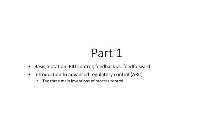
Part 1 Basis, notation, PID control, feedback vs. feedforward Introduction to advanced regulatory control (ARC) The three main inventions of process control

NOTATION and BLOCK DIAGRAMS MV = manipulated variable (controller output) CV = controlled variable (controller input) u = process input (adjustable) d = disturbance y = process output (with setpoint ys) w = extra measured process variable (state x, y2) (non-adjustable) Combine: ? = ?? ?? Block diagrams: All lines are signals (information)

PID control You need a PhD to tune a PID

SIMC PID tuning rule + ?? = filter time constant (on measurement y) k =k/ 1 Only one tuning parameter: Closed-loop time constant: 1 ?? ? (gives Gain Margin>3) Filter time constant, ?? ?? 2 Note: For integrating processes (with large time constant 1): Both Kcand I depend on c Example: Level control (often poorly tuned), ????= 4/?

Motivation for better control: Squeeze and shift rule y

Feedforward control: Measure disturbance (d) dm gdm Process cFd e ym gm Block diagram of feedforward control c = Feedback controller cFd = Feedforward controller. Ideal, inverts process g: ???= ?_?????? _? Usually: Add feedforward when feedback alone is not good enough, for example, because of measurement delay in gm

What is best? Feedback or feedforward?

Example: Feedback vs. feedforward for setpoint control of uncertain process G y = G(s) u

Example: Feedback vs. feedforward for setpoint control of uncertain process G y = G(s) u

But what happens if the process changes? Consider a gain change so that the model is wrong Process gain from k=3 to k =4.5

Gain error (feedback and feedforward): From k=3 to k=4.5 Time delay (feedback): From ? = 0 ?? ? = 1.5

Introduction to Advanced regulatory control (ARC) Uses Flowsheets

The three main inventions of process control (became widely used in the process industry in the 1930s) 1. 2. 3. PID control, and in particular integral action ( bias reset) Cascade control Ratio control (special case of feedforward which needs no explicit model) The last two are used if standard feedback is not good enough, typically because of delay in measurement of y. Cascade: Use extra output measurement (y2) Ratio/feedforward: Use disturbance measurement (d)

Feedback control Flowsheet (P&ID) of feedback control Example: Level control (with given outflow) Inflow (u) Hs H LC Outflow (d) CLASSIFICATION OF VARIABLES FOR CONTROL (MV, CV, DV): INPUT (u, MV): INFLOW OUTPUT (y, CV): LEVEL DISTURBANCE (d, DV): OUTFLOW MV = manipulated vartiable (input u) CV = controlled variable (output y) DV = disturbance variable (d)

Feedback control Level control when inflow is given (alternative input/output-pairing) Inflow (d) Hs H LC Outflow (u) CLASSIFICATION OF VARIABLES FOR CONTROL (MV, CV, DV): INPUT (u, MV): OUTFLOW (Input for control!) OUTPUT (y, CV): LEVEL DISTURBANCE (d, DV): INFLOW

y1 u Process Invention 2. Cascade control y2 y1=primary output (given setpoint) y2=secondary output (adjustable setpoint) Idea: make use of extra local output measurement (y2) Implementation: Controller ( master ) gives setpoint to another controller ( slave ) Without cascade: Master controller directly adjusts u to control primary output y1) With cascade: Local slave controller (fast) uses u to control extra /fast measurement (y2). * Master (slow) controller adjusts setpoint y2s. Example: Flow controller on valve (very common!) y1 = level H in tank u = valve position (z) y2 = flowrate q through valve WITHOUT CASCADE WITH CASCADE flow in flow in Hs Hs y=H y1=H LC LC master MV=z valve position MV=y2s=qs y2=q FC slave measured flow u=z flow out flow out *Comment: Another approach that uses extra measurements to improve control is Full state feedback .

Block diagram of cascade control master slave y = y1= H (measured level) u = z (valve position) w = y2= q (measured outflow) C1= LC (P-controller) C2= FC (I-controller) G1= k /s (level is integrating) G2= valve model (nonlinear, static) d1= downstream pressure d2= inflow flow in Hs y1=H LC master MV=y2s=qs y2=q FC slave u=z flow out

Cascade control What are the benefits of adding a flow controller (slave=inner cascade)? qs Extra measurement y2= q q z 1. (FC reacts faster than outer level loop) Fast local control: Eliminates effect of disturbances in p1 and p2 2. Counteracts nonlinearity in valve, f(z) With fast flow control we can assume q = qs 1 f(z) 0 0 1 z (valve opening)

Cascade control Time scale separation is needed for cascade control to work well Inner loop (slave) should be at least 4 times* faster than the outer loop (master) But normally recommend 10 times faster tauc_master > 10 tauc_slave Otherwise, the slave and master loops may start interacting The fast slave loop is able to correct for local disturbances, but the outer loop does not know this and if it s too fast it may start fighting with the slave loop. This may also result in stability problems * Shinskey (Controlling multivariable processes, ISA, 1981, p.12)

Time-scale separation Response of linear first-order system (with time constant ) y u Block diagram with transfer function for first-order process y(t= ) = k u Convergence rate (of inner loop): 63% after 1 98% after 4 (recommended lower limit) To be safe (process changes): 10

Invention 3. Ratio control Example: Process with two feeds d=q1 and u=q2, where ratio should be constant. Use multiplication block (x): (u/d)s=(q2/q1)s (desired flow ratio) u=q2 (MV: manipulated variable) d=q1 (measured flow disturbance) x

Usually: Combine ratio (feedforward) with feedback Adjust (q1/q2)s based on feedback from process, for example, composition controller. Maybe be viewed a special case of cascade control Example mixing process (cake baking): Use recipe initially (ratio control = feedforward), but adjust ratio if result is not as desired (feedback)

EXAMPLE: RATIO CONTROL FOR MIXING PROCESS Rs= (q2/q1)s q1,m q2,s x FC q1 [m3/s] C1 [mol/m3] q2,m C2=0 Water Concentrate H LC cm c CC q [m3/s] c [mol/m3] cs Diluted product CC: outer cascade = feedback trim (correction) of ratio setpoint Later: Will see that this is a special case of input transformation: Transformed input (as seen from feedback controller CC) is v = (q2/q1)s

The three main inventions of process control can only indirectly and with effort be implemented with MPC 1. Integral action with MPC: Need to add artificial integrating disturbance in estimator ARC: Just add an integrator in the controller (use PID) 2. Cascade control with MPC: Need model for how u and d affect y1and y2. ARC: Just need to know that control of y2indirectly improves control of y1 3. Ratio control with MPC: Need model for how u and d affect property y ARC: Just need the insight that it is good for control of y to keep the ratio R=u/d constant Because of this, MPC should be on top of a regulatory control layer with the setpoints for y2and R as MVs.