Advanced Concepts in Matrices and Computational Physics

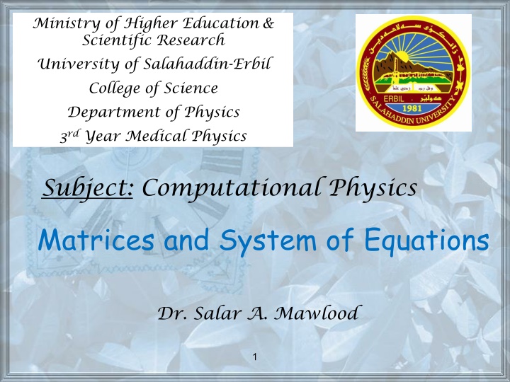
Ministry of Higher Education& Scientific Research University of Salahaddin-Erbil College of Science Department of Physics 3rd Year Medical Physics Subject: Computational Physics Matrices and System of Equations Dr. Salar A. Mawlood 1

Types of Matrices Row Matrix A matrix with order 1 2 1 2 1 n 1 2 Column Matrix A matrix with order 2 1 m 1 Square Matrix A matrix with the same number of rows & column 0 0 0 0 1 2 3 4 2 2 Null (Zero) Matrix , O A matrix where all the elements are zero = Identity Matrix, I A square matrix where the elements in the main diagonal are all 1 s & the others are all zeros 1 0 0 1 = I 2

Diagonal Matrix A square matrix where all its elements zeros, except for those in the main diagonal 0 b a 0 Symmetric Matrix A square matrix where the elements are symmetrical about the main diagonal 1 2 2 4 Upper Triangular Matrix A square matrix where all the elements below the main diagonal are zeros 1 0 3 2 Lower Triangular Matrix A square matrix where all the elements above the main diagonal are zeros 1 3 0 2 3

Basic Properties of Determinants I. The interchange of any two rows will alter the sign but not its numerical value The multiplication of any one row by a scalar k will change its value k-fold The addition of a multiple of any row to another row will leave it unaltered. The interchange of rows and columns does not affect its value If one row is a multiple of another row, the determinant is zero If two rows (columns) are equal, then determinant is zero. II. III. IV. V. VI. 4 4

Matrix of Cofactors & Adjoint matrix a a a a a a a a a c c c c c c c c c 11 12 13 11 12 13 = A C 1. If the matrix of cofactors is , = 21 22 23 21 22 23 31 32 33 31 32 33 a a a a a a a a 22 23 21 23 = = where , and so on c c 11 12 32 33 31 33 2. The transpose of the matrix of cofactors of A is the adjoint matrix, denoted by Adj A c c c c c c T c c c c c c c c c c c c 11 12 13 11 21 31 = = = T A C Adj 21 22 23 12 22 32 31 32 33 13 23 33 5

Matrix inverse A square matrix A is invertible or nonsingular if there exist a square matrix B, called an inverse of A, such that and AB = I ( B ( A BA = I ) ) B is called an inverse of A A is called an inverse of B = = 1 A B 1 An invertible matrix A has only one inverse (The inverse is unique) & is denoted by and AA = I 1 A -1 -1 A A = I When does not exist and A is called noninvertible or singular matrix = 1 A A 0, 6

Ex: Classifying square matrices as singular or nonsingular A square matrix A is invertible (nonsingular) if and only if det (A) 0 1 0 2 1 1 0 2 1 = 3 2 B = 3 2 A 3 2 1 3 2 1 Sol: A has no inverse (it is singular). = 0 A = B has inverse (it is nonsingular). 12 0 B 7

Properties of Inverse If A and B are nonsingular matrices (invertible), ( ) 1 = 1 1 AB B A The inverse of an invertible matrix is also is invertible. So, ( = A ) 1 -1 A Any nonzero scalar product of an invertible matrix is invertible. Also, 1 k ( ) 1 = 1 A A k 1 1= If invertible is A then , det( A ) . det( A ) 8

Find Inverse Matrix by Adjoint Matrix 1 A 0, then has an inverse A A 1. If given by, 1 A 1 A = = 1 T A A C adj where is Cofactor Matrix C A = 2. If det( ) , 0 . then A has no inverse 9

Ex: If 0 1 3 2 = 2 1 A (a) Find the adjoint of A. (b) Use the adjoint of A to find 1 0 2 1 A + + ( 1)i = = j C M Q Sol: ij ij 2 1 0 2 C = + = = + = , 4 2 C 0 1 11 13 0 2 1 0 = = , 1 C 12 1 2 1 3 3 2 1 2 = = = = 3 C , 6 C = + = , 0 C 23 21 1 0 0 2 22 1 2 1 3 3 2 1 2 = + = 2 C = = = + = , 1 C , 7 C 33 0 2 32 31 0 1 2 1 10

4 6 7 1 0 1 2 3 2 4 1 2 6 0 3 7 1 2 T = = C = = = = adj A C ( ) ij ij inverse matrix of A ( ( ) ) A = = Q det 3 1 = = 1 A adj A ( ) ( ( ) ) A det 2 7 4 4 6 7 3 3 = = 0 1 1 1 0 1 1 3 3 3 2 3 2 1 2 2 3 3 1 = AA I Check: 11

Example: Find Inverse Matrix by Adjoint Matrix 4 1 2 = 5 2 1 A 1 0 3 = Determinan t of A 6 6 - 14 - 2 = Cofactors of A - 3 10 1 - 3 6 3 6 - 3 - 3 = Adjoint A - 14 10 6 - 2 1 3 6 - 3 - 3 1 = Inverse of A - 14 10 6 6 - 2 1 3 12 12

Find Inverse Matrix by Elementary Row Operation To find , if it exist, do the following A 1 Find the reduced row echelon form (by elementary row operation) of the matrix [A:I], say [B:C] If B has a zero row, STOP. So, A is noninvertible. Otherwise, go to Step 3. 1 A The reduced matrix is now in the form [I: ]. Read the inverse A 1 13

Elementary Row Operation The elementary row operation of a matrix consist of the following: Elimination : Adding a constant multiple of one row to another + cR R R j i i Scaling : Multiplying a row by a nonzero constant cR R i i Interchange : Interchanging two row R R i j 14

Ex.: Find Inverse Matrix By Elementary Row Operation 0 11 4 1 0 0 2 6 2 0 1 0 swap rows 1 & 3 4 1 0 0 0 1 4 1 0 0 0 1 * 1 4 2 6 2 0 1 0 0 11 4 1 0 0 1 1 4 0 0 0 1 4 * 2 4 + 2 6 2 0 1 0 0 11 4 1 0 0 1 1 4 0 0 0 1 1 0 11 2 2 0 1 1 2 * 2 11 0 11 4 1 0 0 1 1 4 0 0 0 4 0 1 4 11 0 2 11 1 11 * 11 + 0 11 4 1 0 0 1 1 4 0 0 0 1 4 0 1 4 11 0 2 11 1 11 0 0 0 1 2 1 15 15

Ex.: Find Inverse Matrix By Elementary Row Operation 4 1 2 1 0 0 1 0 3 0 0 1 5 2 1 0 1 0 swap rows 1 & 3 0 1 7 0 1 2 5 2 1 0 3 0 0 1 0 0 3 1 1 2 3 2 * 1 3 1 0 3 0 0 1 * 5 + 5 2 1 0 1 0 1 0 3 0 0 1 4 1 2 1 0 0 + 0 1 7 0 1 2 5 2 1 0 3 0 0 1 0 0 1 1 3 1 6 1 2 * 7 0 2 14 0 1 5 * 1 2 + 1 0 3 0 0 1 1 4 1 2 1 0 0 0 1 0 7 3 5 3 1 1 0 3 0 0 * 4 1 0 0 1 1 3 1 6 1 2 * 3 0 1 7 0 1 2 5 2 1 0 0 1 1 2 2 + 4 1 2 1 0 0 0 1 0 7 3 5 3 1 1 0 3 0 0 1 0 0 1 1 3 1 6 1 2 0 1 7 0 1 2 5 2 * 1 + 0 1 10 1 0 4 16 16

Ex: Which of the following system has a unique solution? (a) (b) = 2 1 x x = 2 1 x x 2 3 2 3 + = 3 2 4 x x x + = 3 2 4 x x x 1 2 3 1 2 3 + = 3 2 4 x x x + + = 3 2 4 x x x 1 2 3 1 2 3 0 3 3 2 1 x = A b Sol: = = = = A Q 2 1 0 2 1 This system does not has a unique solution. x = B b B = = Q 12 0 This system has a unique solution. 17

Solving for x using Matrix Inversion adjA = = * Ax d x d A x d C C C 1 1 11 21 1 n x d C C C 2 2 1 12 22 2 n = A C C C 1 2 x d n n nn n n Q.1: Use Gaussj model for solving the system of equations. (H.W.) Q.2: Use LU decomposition for solving the system of equations. (H.W.) 18 18

Ex: Use Cramers rule to solve the system of linear equations. + = 2 3 1 x y z + = 2 0 x z + = 3 4 4 2 x y z Sol: 1 2 3 1 2 3 = = det( ) 0 0 1 8 A = = det( ) 2 0 1 10 A 1 2 4 4 3 1 4 4 1 3 1 2 1 = = = = det( ) 2 0 0 16 A det( ) 2 0 1 15 , A 3 2 3 4 2 3 2 4 det( ) 8 A det( ) 3 A A A det( det( ) ) 4 5 = = = = z 3 y 2 = = = = x 1 det( ) 5 A det( ) 2 A 19

Example: Find x,y and z from Ax=d Matrix = Ax Inversion Cramer' = Ax Rule s d d 4 1 2 x 4 4 1 2 x 4 = = = 5 2 1 ; x y d ; 4 A = = = 5 2 1 ; x y d ; 4 A A 1 0 3 z 3 1 0 3 z 3 = 1 x d = ; 6 = A 6 - 3 - 3 1 = 1 - A - 14 10 6 = = ; 3 ; 2 ; 5 A A A 6 1 = 2 3 - 2 1 3 = 1 2 x A A 1 x 6 - 3 - 3 4 = = 1 3 y A A 1 2 = y - 14 10 6 4 = = 6 5 6 z A A x z - = 2 1 3 3 3 = = 1 y ; 2 1 3; z 5 6 20 20

Special Matrices Bra-Ket Notation Matrices Vector Xn can be represented by two ways Ket |n> Bra <n| = |n>T ( ) v * * * * * v w x y z w x * m is the complex conjugate of m. y z 21

Inner Products An Inner Product is a Bra multiplied by a Ket <a| |b> can be simplified to <a|b> l m ( ) + + + + * * * * * * * * * * lv mw nx oy pz = v w x y z <a|b> = n o p 22

Outer Products An Outer Product is a Ket multiplied by a Bra l * * * * * lv lw lx ly lz m * * * * * mv mw mx my mz ( ) n * * * * * nv nw nx ny nz * * * * * |a><b| = = v w x y z o * * * * * ov ow ox oy oz p * * * * * pv pw px py pz ( ) = a b c b c a By Definition 23

Pauli Matrices 1 0 0 0 1 0 i i = = = 3 1 2 0 1 1 0 These are the Pauli matrices were introduced to describe a particle of spin (1/2). They are satisfied the following properties: = ) 1 i ...Cyclic permutation of indices l m ) n ( = 2 ) 2 ...Identity I l + = ) 3 2 I ...Anticommutation l m m l lm 24

Dirac Matrices We can build up a complete set of Dirac matrices as direct products of the Pauli matrices and the unit matrix: I a Pauli l Dirac l = , , ) e.g. = ) , , b I l Dirac l Pauli 1 0 1 0 = I , 1 , 1 Pauli Pauli = = , 1 , 1 Dirac Pauli , 1 Pauli 0 1 0 1 , 1 , 1 Pauli Pauli 0 1 0 0 0 i 0 0 i 1 0 0 0 1 0 0 0 0 0 0 i 0 1 0 0 = = = 1, Dirac 2, Dirac 0 0 0 1 3, Dirac 0 0 0 i 0 0 1 0 0 0 1 0 0 0 0 0 0 0 1 25

e.g. 0 1 0 1 I I = I = = I 0 , 1 , 1 Dirac Pauli 1 0 1 0 I I 0 0 1 0 0 0 i i 1 0 0 0 0 0 0 1 0 i 0 0 0 1 0 0 = = = 1, Dirac 2, Dirac 1 0 0 0 3, Dirac 0 i 0 0 0 0 1 0 0 1 0 0 0 0 0 0 0 0 1 We can show that these 4x4 matrices satisfy the relations: = ) 1 i l m n Cyclic permutation of indices = i l m n = 2 = ) 2 [ , ] 0 Commutation l m m l l m + = ) 3 I l m m l lm Anticommutation + = 2 I l m m l lm 26

Orthogonal Matrices Definition: A square matrix A with the property A-1=AT is said to be an orthogonal matrix. Ex.1: A Rotation Matrix is Orthogonal The standard matrix for the counterclockwise rotation of R2 through an angle is cos sin sin cos = A This matrix is orthogonal for all choices of , since cos sin sin cos cos sin sin cos 1 0 0 1 = = T A A 1/ 2 1/ 2 Q. Is the matrix A orthogonal? = A 1/ 2 1/ 2 It is orthogonal since its row (and column) vectors form orthonormal sets in R2 27

Ex.2: The matrix 3/7 6/7 3/7 2/7 2/7 6/7 2/7 3/7 = A 6/7 is orthogonal, since 3/7 6/7 2/7 2/7 3/7 6/7 6/7 2/7 3/7 3/7 6/7 2/7 2/7 3/7 6/7 6/7 2/7 3/7 1 0 0 0 1 0 0 0 1 = = T A A Ex.3: If A is Orthogonal Matrix, show that det[A]= 1 AAT= I a matrix A is said to be orthogonal if: = AAT = T det( ) det( ) I det( A ) det( ) 1 A A = 1 AT ) A But: det( ) det( ) 2= = (det (det ) 1 A 28

Symmetric Matrices Definition A symmetric matrix is a matrix that is equal to its transpose. The transpose of a matrix A, denoted AT, is the matrix whose columns are the rows of the given matrix A. e.g. match 1 0 2 4 0 1 4 2 5 0 7 3 9 1 7 8 5 4 2 3 2 3 4 8 3 4 9 3 6 29

Ex: Let A and B be symmetric matrices of the same size. Prove that the product AB is symmetric if and only if AB = BA. *We have to show (a) if AB is symmetric, then AB = BA, and the converse, (b) AB = BA, then AB is symmetric. Proof (a) Let AB be symmetric, then AB= (AB)T =BTAT = BA (b) Let AB = BA, then (AB)T = BTATby the transpose of a product = BA since A and B are symmetric matrices = AB by definition of symmetric matrix by the transpose of a product since A and B are symmetric matrices 30

Ex: is symmetric T AA Show that Pf: = = T T T T T T ( ) ( ) AA A A AA T symmetric is AA Ex: 1 a 2 3 = is symmetric, find a, b, c? If 4 c 5 A 6 b Sol: 1 a 2 3 1 a b A = T A = = 4 c 5 A AT 2 4 c = , 3 = = , 2 5 a b c 6 b 3 5 6 31

Skew-symmetric matrix: A square matrix S is skew-symmetric if ST = S S R A + = 1 , Any square matrix A may be written as the sum of symmetric & skew-symmetric matrices ( ) = + T R A A symmetric 2 ( ) 1 = T S A A skew symmetric 2 Ex: 0 a 1 2 = is a skew-symmetric, find a, b, c? If 0 c 3 A 2 0 b Sol: 0 a b = 0 a 1 T A A = = = AT 0 c 3 A 1 0 c = , 1 , 2 = 3 a b c 0 b 2 3 0 32

Special Matrices and Their Eigenvalues A real symmetric matrix is one where A = AT. This also includes real diagonal matrices. The eigenvalues and eigenvectors of such matrices are always real Eigenvectors corresponding to distinct eigenvalues are orthogonal Any symmetric matrix is diagonalizable Orthogonal diagonalization For every n x n real symmetric matrix A, there exists an n x n real orthogonal matrix Q such that Q-1AQ = QTAQ= where is a diagonal matrix When this principle holds, the matrix A is said to be orthogonally diagonalizable. This is also called the principal axis theorem in geometry or mechanics. 33

Unitary, Normal, And Hermitian Matrices If A and B are matrices with complex entries and k is any complex number, then the properties of conjugate transpose (H) are: H H A b A A a = ( ) ( ) ( ) ( = + = + H H H ( ( ) ) ( ( ) ) B A B = * H H H H H k kA c ) A d AB B A Definition A square matrix A with complex entries is called Hermitian if A=AH Definition A square matrix A with complex entries is called unitary if 1 = H A A Definition A square matrix A with complex entries is called normal if AAH= AHA 34

Properties of Hermitian Matrices The matrix with complex elements that plays the role of a symmetrical matrix is called Hermitian These matrices are equal to their conjugate transpose, i.e. AH = A A Hermitian matrix has real eigenvalue Eigenvectors of different eigenvalues are orthogonal to one another, i.e., their scalar product is zero. It is also diagonalizable If A is real and Hermitian it is said to be symmetric, & A = AT. Every Hermitian matrix is positive definite. The complex equivalent of an orthongonal matrix is the unitary matrix where UH = U-1. Thus, = U-1AU = UHAU 35

Summary For matrices with real entries, the orthogonal matrices(A-1=AT) and the symmetric matrices(A=AT) played an important role in the orthogonal diagonal-ization problem. For matrices with complex entries, the orthogonal and symmetric matrices are of relatively little importance; they are superseded by two new classes of matrices, the unitary and Hermitian matrices, which we shall discuss in this section. Real matrices Symmetric Skew Symmetric Orthogonal AT=A AT =-A Imaginary or zero eigenvalues QT=Q-1 All | i| = 1 Real eigenvalues Complex matrices Hermitian Skew Hermitian AH=-A Unitary AH=A Real eigenvalues Imaginary or zero eigenvalues UH=U-1 All | i| = 1 36

EXAMPLE: Show that (a) Every eigenvalue of an Hermitian matrix is real. (b) Different eigenvectors of an Hermitian matrix corresponding to two distinct eigenvalues are orthogonal to each other. Let i and j be two eigenvalues and |ri> and |rj> the corresponding eigenvectors of a Hermitian matrix, then: = = nd A r r 2 : . Taking H of eq r A r r r i i i j i i j i = * H = r A r r r A r r = r A r AH= r r j i j j i j j j i j j i j A For Hermitian matrix, = = * r A r r r r r = * ( ) 0 r r j i j j i i j i j i j i = = * ( ) 0 a if i j r r is real i i i i i = * ( ) ( ) 0 0 b if i j r r they are orthogonal i j i j 37

EXAMPLE: A 3 3 Hermitian Matrix 1 i 1 i i If i then i - 2 i + 1 1 i i = 2 + 3 * i 5 i 2 i A = i 5 A + 1 + 1 2 3 so + i - 2 1 1 i i = = 2 = * H T ( ) 5 A A i A + 1 3 i i EXAMPLE: Every Hermitian matrices A is normal since AAH=AA= AHA, and every unitary matrix A is normal since AAH=I= AHA. 38

Physical Applications of Hermitian Matrices An operator O is Hermitian if and only if: * = *) ( , ) ( , f O g g O f = * * ( ) ( ) (4.2) f Og dx g Of dx for all functions f, g vanishing at infinity. * = M M Compare the definition of a Hermitian matrix M: ij ji Analogous if we identify a matrix element with an integral: * ( ) f Of dx M i j ij 39 39