Understanding Spin Magnetism in NMR: An Introduction to Angular Momentum and Magnetic Moments
Delve into the world of spin magnetism in NMR as we explore the concepts of angular momentum, magnetic moments, Stern-Gerlach experiments, and the quantization of spin. Learn about spin projections, spin relaxation, and the relationship between spin particles and external magnetic fields.
Download Presentation

Please find below an Image/Link to download the presentation.
The content on the website is provided AS IS for your information and personal use only. It may not be sold, licensed, or shared on other websites without obtaining consent from the author. Download presentation by click this link. If you encounter any issues during the download, it is possible that the publisher has removed the file from their server.
E N D
Presentation Transcript
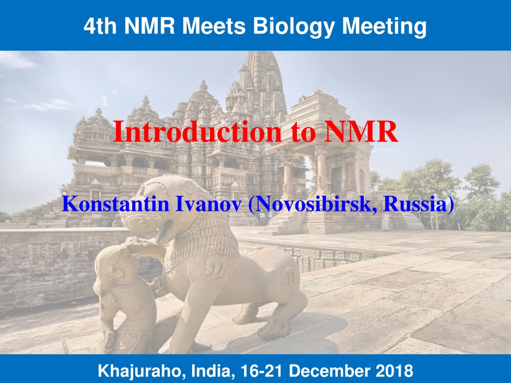
4th NMR Meets Biology Meeting Introduction to NMR Konstantin Ivanov (Novosibirsk, Russia) Khajuraho, India, 16-21 December 2018
Outline Angular moment (spin) and magnetic moment; Magnetic resonance phenomenon; Bloch equations; NMR pulses; FID, Fourier transform, 1D-NMR, 2D-NMR; T1and T2relaxation. 2
Angular momentum and magnetic moment In NMR we deal with spin magnetism. What is spin ? Charged nucleus (or electron) is spinning: there is angular momentum (spin) and magnetic moment attention: this is a simple view, which is not (entirely) correct qv 2 = I The electric current for a charged particle moving around r q IS qvr 2 q = = = The magnetic moment is n n J mc 2 c c q = S So, is proportional to a.m.; when a.m. is measured in units 2 mc Quantum mechanics: this is not entirely correct (we are wrong by the g-factor)! e = = = + + , , 2 1 ... . 2 0023 ( QED result ) g S g e e B B e 2 2 m c e 2 e = = = , , 1 ( . 5 58 , . 3 83 , QCD result ) g I g g g g 3 N N N N N p n p 2 3 Mc
Angular momentum and magnetic moment Furthermore, QM tells us that S is quantized: angular moment measured in units cannot be an arbitrary number Stern-Gerlach experiment: The beam of particles is deflected by inhomogeneous field Reason: intrinsic magnetic moment (spin) of particles In contrast to the classical expectation the distribution of the -vector is not continuous! Spin is quantized 4
Angular momentum and magnetic moment Furthermore, QM tells us that S is quantized: angular moment measured in units cannot be an arbitrary number S is integer (0, 1, 2, ) or half-integer (1/2, 3/2, 5/2, ) and |S|={S(S+1)}1/2 Projection of S onto any axis in space varies in steps of 1 from S to S Spin- particle (1H, 13C, 15N, 19F, 31P ): possible projections are 1/2 Spin-1 particle: possible projections are 1, 0, 1 When discussing spin- particles we can use a simplification (and forget about QM): spin magnetization is a classical vector in the 3D-space, which is changing by moving in external fields and due to spin relaxation As we can see from the density matrix description, this is correct (but only for two-level systems!): fictitious spin description 5
Magnetic resonance: classical viewpoint Motion of a classical magnetic moment in a constant magnetic field B0 = = g J J Magnetic moment is Nis the gyromagnetic ratio (or magnetogyric ratio) N N N N B0 d J We obtain a torque: = = B J B torque 0 0 N dt , J dJ dJ y = = = , , const B J B J J x 0 0 N y N x z dt dt ( ) ( ) = These equations tell us that: |J|=const; the J-vector is rotating about B0at a frequency 0=| N|B0 This is precession of magnetic moment The direction is given by the Nsign What happens to the magnetic moment if we apply an oscillating field? Typically this field is much weaker than B0: it does nothing except for some special cases cos , sin , const J t J t J 0 0 x y z 6
Magnetic resonance: classical viewpoint Let us apply an oscillating field perpendicular to B0: B =2B1cos( t) To account for the effect of this field we can go to the rotating frame: , sin ' cos ' t y t x y = If a is a constant vector in the RF, in the LF we obtain z=z = + x x t y t d a = [ ] = + a ' sin ' cos , y dt ' z z t y x x Linear polarized field = 2 circularly polarized fields: two vectors rotating with the same speed in opposite directions y y Rot. frame Lab frame x x At high the vector, which rotates with double frequency can be neglected. This is (usually) Ok for the description of resonance 7
Magnetic resonance: classical viewpoint = ) 0 , 0 , t What happens to the transverse field: 2 cos 2 (cos B t B 1 1 Linear polarized field = 2 circularly polarized fields: two vectors rotating with the same speed in opposite directions (cos( ) 0 , sin , (cos 1 1 B t t B + ), sin( ) 0 ), t t Graphical representation in both frames: y y Lab frame Rot. frame x x At high the vector, which rotates with double frequency can be neglected. The other vector does not move. This is (usually) Ok for the description of resonance 8
Magnetic resonance: classical viewpoint Equation of motion in the rotating frame ' ' + = Here the components of J change and the basis vectors {i, j, k} also change with time + ' J J i J j J k x y z By taking derivative we obtain: + = ' y dJ ' x ' z dJ d J dJ + + i j k Here / t is the time derivative in the rotating frame dt dt dt dt i d j d d k J + + + = + ' x ' y ' z [ ] J J J J dt dt dt t Equation of motion in the rotating frame = = J d J + = [ ] [ ] [ ] [ ] J J B J J B N N eff t dt = + + / B B B Still the same equation but the new field equals to 0 1 eff N Superposition of the new B0and B1-fields gives a constant effective field Beff 9
Magnetic resonance: classical viewpoint = ( ( , 0 , 1 B / ) 0 ) B The effective field is the following vector eff N z Beff Precession frequency is B0 /| | = = + 2 2 1 ( 0) NB x eff B1 If = 0the precession axis is the x-axis => variation of Jzreaches its maximum. This variation rapidly decays with going to zero at | 0|>> 1 Resonance condition: = (free precession frequency). Weak B1is important! Frequency range (given by N): radio-frequency, i.e., 300 MHz for 1H @ 7 Tesla Resonance width is given by condition | 0| 1. If 1>>| 0| the effective field is nearly parallel to the x-axis we are at resonance! At resonance the precession frequency is 1. If we switch on the resonant oscillating field for time period of pthe flip angle of magnetization is 1 = = B 1 p N p 10
Magnetic resonance: simplified quantum viewpoint The energy of interaction of the spin with an external field is H N = ) I = ( ) ( B B 0 0 N = E B I If B0is parallel to the Z-axis 0 N z The degeneracy of the spin levels is lifted E=| N|B0/2 = / 1 2 Periodic perturbation Absence of MF H F I = = 2 ( ) 2 cos cos t t B t 1 N x E= | N|B0/2 = / 1 2 Presence of MF Fermi golden rule tells us that there is a resonance when = 0 ( 2 2 = 2 1 ) ( ) P F E E B 0 11
Macroscopic spin magnetization Up to now we discussed a single spin , which is never the case in NMR At thermal equilibrium we have almost the same amount of spins pointing up and down: the energy gap between the spin levels is much smaller than kT B0 = = M B Nuclear paramagnetism: the induced field is parallel to B0 0 i i ) 1 + 2 2 ( N I I = N kT 3 We work with net magnetization of all spins; at equilibrium this is a vector parallel to B0(longitudinal magnetization) However, we do not measure the longitudinal component, but rotate M with RF pulses to obtain transverse magnetization and measure the signal from M 12
T1and T2relaxation Relaxation is a process, which brings a system to thermal equilibrium. Physical reason: fluctuating interaction of spins with molecular surrounding For spins this means that Mz=M||=Meqand M =0 There are two processes, which are responsible for relaxation Longitudinal, T1, relaxation: Meqis reached at t~T1: ( M M M eq eq z = ) exp( / ) M t T 0 1 Transverse, T2, relaxation: magnetization decays to zero at t~T2: exp( 0 M M = / ) t T 2 Generally, T1 T2. Taking all that into account we can write down equations describing precession+relaxation 13
Bloch equations and FID We write down equations describing precession and add relaxation terms ) ( / M M dt dM x y x = = / , T 0 2 M / ( ) / , dM dt M M T 0 M 1 2 y x z y = / ( / ) eq dM dt M M T 1 1 z y z Now we can describe simplest NMR experiments. Example: Mzis flipped by 90 degrees by a resonant RF-pulse: = 1 p= /2 It starts rotating about the z-axis and decaying with T2 We detect My(or Mx) and collect the Free Induction Decay (FID) = ( ) cos( ) exp( / ) M t M t t T 0 0 2 z How to obtain the spectrum? 1 y 0 t -1 Free Induction Decay 14 x
Fourier Transform NMR How do we obtain the spectrum by performing the Fourier transform 0 g( ) = f(t) cos( t)dt Fourier transform 1 0 t -1 time domain f(t) frequency domain g( ) Some examples cos( ) ( ) 0t FT -function, single freq. 0 T = t ( ) L 2 Lorentzian at zero freq. exp( / ) 2 T FT + 2 2 1 T 2 Lorentzian at 0freq. ( ) L cos( ) exp( / ) M t t T FT 0 0 0 2 15
Fourier Transform NMR How do we obtain the spectrum by performing the Fourier transform 0 g( ) = f(t) cos( t)dt Fourier transform 1 0 t -1 time domain f(t) frequency domain g( ) Some examples ( = ( ) g FID ( ) cos( ) d ) t t g FT Inverse FT gives g( ) from the FID signal ( ) g FID t ( ) IFT Widths of g( ) and FID(t) are inter-related: t~1/ FT can be performed in a fast and efficient way (FFT algorithm) 16
Fourier Transform NMR A few words about pulses RF-synthesizer produces a signal oscillating at the spectrometer reference frequency ref: ( ( cos ) ( t t t S ref + can be precisely controlled ) ) The phase is time-dependent and Gating: the signal passes through the transmitter only for certain periods of time => we obtain an RF-pulse 1 1 1 0 0 0 -1 -1 -1 Parameters of the pulse: frequency ref strength B1and duration pprovide the flip angle = | N|B1 p = 1 p phase: =0 (x-pulse), = /2 (y-pulse), = ( x-pulse), =3 /2 ( y-pulse) 17
Fourier Transform NMR A few words about FID detection We measure the signal comparing it to the reference frequency ref (recording oscillations at ~100 MHz frequency would be a disaster) 0 0 = 0 ref / / t T t T ( ) cos( 0) t ( ) cos( 0) t M t e M t e 2 2 Problem: no sensitivity to the sign of 0( ref greater or smaller than 0) The solution is quadrature detection: the receiver provides a phase-shifted signal to obtain the information about the sign / 0 , ) cos( ) ( A S e t C t S = = / t T t T ( ) sin( ) t C t e 2 2 0 B We introduce complex magnetization , which contains full information ) ( ) ( ) ( t S i t S t S B A = + = ( ) exp / C i t t T 0 2 ( ) 0 i = i t ( ) exp / S C t t T e dt Fourier transformation yields 0 2 Yet phasing is a problem 18
Fourier Transform NMR ( ) 0 i = i t ( ) exp / S C t t T e dt Fourier transformation yields 0 2 Real and imaginary part of the signal (when C is real) T = = Re ( ) ( ) S L 2 L( ) ( ) 0 2 + 2 1 T 0 2 T ( ) 2 = = Im ( ) ( ) S D 0 2 ( ) 0 2 + 2 1 T D( ) 0 2 Generally, C=|C|ei is a complex number because of a phase shift of the pulser and receiver cos ) ( ) ( Re 0 D L S ( ) sin 0 By varying the phase we can obtain the Lorenzian or purely dispersive line The phase can be set and then kept the same 19
Back to relaxation Before talking about 2D-NMR let us briefly discuss T1and T2 Origin of T1and T2 Relaxation and molecular motion Measurement of the relaxation times 20
T1-relaxation T1-relaxation: precession in the B0field and a small fluctuating field Bf (t) B0 B0 B0+Bf (t) The precession cone is moving Eventually, the spin can even flip Spin flips up-to-down and down-to-up have slightly different probability (Bolztmann law!): Mzgoes to Meq 0 1 T 1 2 General expression for the transition rate = = ( ) W V J 2 2 1 2 + Noise spectral density at the transition frequency cis the motional correlation time = ( ) J c 2 2 c 1 21
T2-relaxation T2-relaxation: kicks from the environment disturb the precession Different spins precess differently and transverse net magnetization is gone Dephasing Generally the T2-rate Two contributions: Adiabatic and non-adiabatic (T1-related) 1 T 1 1 na 1 1 T = + = + a a 2 T T T 2 2 2 2 1 22
Noise spectral density Simple example: spins relaxed by fluctuating local fields, Bf (t)=0 However, the auto-correlation function is non-zero t + = ( ( ) ( ) ) f t f t G time Typical assumption 1.0 Exponential auto-correlation function ccomes into play = ( ) exp( | / | ) G 0.8 c 0.6 G(t) 0.4 0.2 0.0 0 1 2 3 4 5 t/ c Lorentzian-like noise spectral density 2 + J( ) = = i t ( ) 2 ( ) d J G t e t c 2 2 c 1 0 23
Expressions for T1and T2 Simple example: spins relaxed by fluctuating local fields, Bf (t)=0 The auto-correlation function is non-zero General expressions for T1and T2 c c ( ) 1 = + 2 * 2 * 2 , c B B x y + 2 2 1 T T1 1 c + 2 2 1 c T 1 c c c This dependence is explained by the J( ) behavior 1 T 1 1 na 1 1 T 1= = + = + 2 * 2 B z c a a 2 a T T T T 2 2 2 2 1 2 24
Inhomogeneous linewidth Problem: we need to discriminate two contributions to T2 Decay of the NMR signal also proceeds due to static inhomogeneities in the precession frequency 0. This can be due to external field gradients and local static interactions. NMR spectrum Resulting rate the signal decay 1 1 1 1 = + + + Reason: t~2 * a na 2 T T T T 2 2 2 The first two contributions are the same for all the molecules and thus define the homogeneous linewidth. The last contribution defines the inhomogeneous linewidth. In solids usually 2 2 T T * 25
T2-measurement: spin echo Large inhomogeneous linewidth means very fast dephasing of the spin However, dephased magnetization can be focused back by pulses echo /2 pulse sequence /2x- - x t 2 0 Explanation: let us divide system into isochromates having the same frequency 0. Their offsets are = 0 . At certain time they all have different phases t=0 =0 = + (t ) = t t=2 = y y y y x x x x But at t=2 all have the same phase: there is an echo ! The spin echo signal decays with T2 26
T1-measurement: inversion-recovery Determination of T1is often quite important as well Standard method is inversion-recovery First we turn the spin(s) by pulse (usually /2 or ) and then look how system goes back to equilibrium (recovers z-magnetization). If the pulse is a -pulse magnetization will be inverted (maximal variation of m-n) and then recovered Equation for Mzis as follows: ) ( t M z = ( ) ( ) exp / M M M t T 1 0 1 eq eq t 1 The kinetic trace (t-dependence) gives T1-time To detect magnetization at time t one more /2-pulse is applied, the sequence is then x- t (variable) - x/2 - measurement Spin echo can be used for detection as well, the pulse sequence is then x- t (variable) - x/2 - - x- - measurement The sequence should be repeated with different delays t
1D-NMR 1D-NMR experiment (simplest case) FT S(t) S( ) preparation - detection Why is it not enough? For large proteins it is really hard to assign NMR signals and to obtain information from the spectra! Too many peaks Spectrum is a mess! 28
2D-NMR Idea: adding a second dimension for improved resolution FT1, FT2 2D FT-NMR implementation S(t1,t2) S( 1, 2) t2 t2 direct domain t1 indirect domain t1 tm Preparation evolution mixing detection It is up to you how to design preparation and mixing: decide, what you want to know about your molecules! 29
2D-NMR spectrum of a protein Contour plot: topographical lines In 2D the peaks become resolved 30
Direct and indirect domain Direct time domain (acquisition, t2): FID detection Indirect time domain (evolution time, t1in 2D): FIDs are collected for different t1times FT (t2) w1 w2 FT (t1) t2=0 t2 t1 The FID depends on the evolution in t1: the signal is 'modulated' with 1 For simplicity here the frequency is the same in t1and in t2 31
Cross-peaks and diagonal peaks Simple example: SCOTCH experiment Spin COherence Transfer in (photo) CHemical reactions h ReactionA B with a proton at Ain A which resonates at Bin B. l i g h t t1 t2 FT M magnetization evoilves with the frequency Ain t1. After the light pulse, the frequency changes to B. FT provides a 2D spectrum with a peak at Ain F1and Bin F2 The cross-peak comes from A B and A B When conversion A B is incomplete the diagonal peak stays 32
Example: NOESY experiment /2 /2 /2 Cross-peaks come from NOE during the mixing period t1 tm t2 SY = SpectroscopY How does it work? /2x /2x NOE /2x t1 I1z I1y I1y I1z I2z I2y Transverse magnetization has gone from spin 1 to spin 2 The efficiency of transfer is (simplified) sin( 1t1) *sin( 2t2) 1 2 1 A cross-peak will appear in the NOESY-spectrum The cross-peak gives information on NOE distance between the spins The same method can be used to study chemical exchange (EXSY) 33
Summary NMR is working with magnetic moments of nuclei (originating from their spins) Simple theory (Bloch equations) allows one to understand basic experiments 1D & 2D NMR concepts are introduced 34
