Understanding Neural Network Learning and Perceptrons
Explore the world of neural network learning, including topics like support vector machines, unsupervised learning, and the use of feed-forward perceptrons. Dive into the concepts of gradient descent and how it helps in minimizing errors in neural networks. Visualize the process through graphical examples to enhance your understanding.

Download Presentation

Please find below an Image/Link to download the presentation.
The content on the website is provided AS IS for your information and personal use only. It may not be sold, licensed, or shared on other websites without obtaining consent from the author. Download presentation by click this link. If you encounter any issues during the download, it is possible that the publisher has removed the file from their server.
E N D
Presentation Transcript
Learning II Linda Shapiro CSE 455 1
More on Learning Neural Nets Support Vectors Machines Unsupervised Learning (Clustering) K-Means Expectation-Maximization
Neural Net Learning Motivated by studies of the brain. A network of artificial neurons that learns a function. Doesn t have clear decision rules like decision trees, but highly successful in many different applications. (e.g. face detection) We use them frequently in our research. I ll be using algorithms from http://www.cs.mtu.edu/~nilufer/classes/cs4811/2016- spring/lecture-slides/cs4811-neural-net-algorithms.pdf 3
Simple Feed-Forward Perceptrons in = ( Wj xj) + out = g[in] W1 x1 out g(in) g is the activation function x2 W2 It can be a step function: g(x) = 1 if x >=0 and 0 (or -1) else. It can be a sigmoid function: g(x) = 1/(1+exp(-x)). The sigmoid function is differentiable and can be used in a gradient descent algorithm to update the weights.
Gradient Descent takes steps proportional to the negative of the gradient of a function to find its local minimum Let X be the inputs, y the class, W the weights in = Wj xj Err = y g(in) E = Err2 is the squared error to minimize E/ Wj = Err * Err/ Wj = Err * / Wj(g(in))(-1) = -Err * g (in) * xj The update is Wj <- Wj + * Err * g (in) * xj is called the learning rate.
Simple Feed-Forward Perceptrons repeat for each e in examples do in = ( Wj xj) + Err = y[e] g[in] Wj = Wj + Err g (in) xj[e] until done W1 x1 out g(in) x2 W2 Examples: A=[(.5,1.5),+1], B=[(-.5,.5),-1], C=[(.5,.5),+1] Initialization: W1 = 1, W2 = 2, = -2 Note1: when g is a step function, the g (in) is removed. Note2: later in back propagation, Err * g (in) will be called We ll let g(x) = 1 if x >=0 else -1
Graphically Examples: A=[(.5,1.5),+1], B=[(-.5,.5),-1], C=[(.5,.5),+1] Initialization: W1 = 1, W2 = 2, = -2 W2 Boundary is W1x1 + W2x2 + = 0 wrong boundary A C B W1
repeat for each e in examples do in = ( Wj xj) + Err = y[e] g[in] Wj = Wj + Err g (in) xj[e] until done Examples: A=[(.5,1.5),+1], B=[(-.5,.5),-1], C=[(.5,.5),+1] Initialization: W1 = 1, W2 = 2, = -2 Learning A=[(.5,1.5),+1] in = .5(1) + (1.5)(2) -2 = 1.5 g(in) = 1; Err = 0; NO CHANGE Let =.5 B=[(-.5,.5),-1] In = (-.5)(1) + (.5)(2) -2 = -1.5 g(in) = -1; Err = 0; NO CHANGE W1 <- W1 + .5(2) (.5) leaving out g <- 1 + 1(.5) = 1.5 W2 <- W2 + .5(2) (.5) <- 2 + 1(.5) = 2.5 <- + .5(+1 (-1)) <- -2 + .5(2) = -1 C=[(.5,.5),+1] in = (.5)(1) + (.5)(2) 2 = -.5 g(in) = -1; Err = 1-(-1)=2
Graphically Examples: A=[(.5,1.5),+1], B=[(-.5,.5),-1], C=[(.5,.5),+1] Initialization: W1 = 1, W2 = 2, = -2 W2 a Boundary is W1x1 + W2x2 + = 0 wrong boundary A C B W1 approximately correct boundary
p1 vector W b error new W
Back Propagation Simple single layer networks with feed forward learning were not powerful enough. Could only produce simple linear classifiers. More powerful networks have multiple hidden layers. The learning algorithm is called back propagation, because it computes the error at the end and propagates it back through the weights of the network to the beginning.
(slightly different from text) Let s break it into steps.
Lets dissect it. layer 1 2 3=L w11 x1 n1 w1f w21 nf x2 w31 w2f n2 x3
Forward Computation layer 1 2 3=L w11 x1 n1 w1f w21 nf x2 w31 w2f n2 x3
Backward Propagation 1 input sum to get the change delta. Node nf is the only node in our output layer. Compute the error at that node and multiply by the derivative of the weighted layer 1 2 3=L w11 x1 n1 w1f w21 nf x2 w31 w2f n2 x3
Backward Propagation 2 At each of the other layers, the deltas use the derivative of its input sum the sum of its output weights the delta computed for the output error layer 1 2 3=L w11 x1 n1 w1f w21 nf x2 w31 w2f n2 x3
Backward Propagation 3 Now that all the deltas are defined, the weight updates just use them. layer 1 2 3=L w11 x1 n1 w1f w21 nf x2 w31 w2f n2 x3
Back Propagation Summary Compute delta values for the output units using observed errors. Starting at the output-1 layer repeat propagate delta values back to previous layer update weights between the two layers till done with all layers This is done for all examples and multiple epochs, till convergence or enough iterations.
Time taken to build model: 16.2 seconds Correctly Classified Instances 307 80.3665 % (did not boost) Incorrectly Classified Instances 75 19.6335 % Kappa statistic 0.6056 Mean absolute error 0.1982 Root mean squared error 0.41 Relative absolute error 39.7113 % Root relative squared error 81.9006 % Total Number of Instances 382 TP Rate FP Rate Precision Recall F-Measure ROC Area Class 0.706 0.103 0.868 0.706 0.779 0.872 cal 0.897 0.294 0.761 0.897 0.824 0.872 dor W Avg. 0.804 0.2 0.814 0.804 0.802 0.872 === Confusion Matrix === a b <-- classified as 132 55 | a = cal 20 175 | b = dor
Kernel Machines A relatively new learning methodology (1992) derived from statistical learning theory. Became famous when it gave accuracy comparable to neural nets in a handwriting recognition class. Was introduced to computer vision researchers by Tomaso Poggio at MIT who started using it for face detection and got better results than neural nets. Has become very popular and widely used with packages available. 27
Support Vector Machines (SVM) Support vector machines are learning algorithms that try to find a hyperplane that separates the different classes of data the most. They are a specific kind of kernel machines based on two key ideas: maximum margin hyperplanes a kernel trick 28
The SVM Equation ySVM(xq) = argmax i,c K(xi,xq) c i=1,m xq is a query or unknown object c indexes the classes there are m support vectors xi with weights i,c, i=1 to m for class c K is the kernel function that compares xi to xq
Maximal Margin (2 class problem) In 2D space, a hyperplane is a line. margin In 3D space, it is a plane. hyperplane Find the hyperplane with maximal margin for all the points. This originates an optimization problem which has a unique solution. 30
Support Vectors The weights i associated with data points are zero, except for those points closest to the separator. The points with nonzero weights are called the support vectors (because they hold up the separating plane). Because there are many fewer support vectors than total data points, the number of parameters defining the optimal separator is small. 31
Kernels A kernel is just a similarity function. It takes 2 inputs and decides how similar they are. Kernels offer an alternative to standard feature vectors. Instead of using a bunch of features, you define a single kernel to decide the similarity between two objects. 33
Kernels and SVMs Under some conditions, every kernel function can be expressed as a dot product in a (possibly infinite dimensional) feature space (Mercer s theorem) SVM machine learning can be expressed in terms of dot products. So SVM machines can use kernels instead of feature vectors. 34
The Kernel Trick The SVM algorithm implicitly maps the original data to a feature space of possibly infinite dimension in which data (which is not separable in the original space) becomes separable in the feature space. Feature space Rn Original space Rk 1 1 1 0 0 0 1 0 0 1 0 0 Kernel trick 1 0 0 0 1 1 35
Kernel Functions The kernel function is designed by the developer of the SVM. It is applied to pairs of input data to evaluate dot products in some corresponding feature space. Kernels can be all sorts of functions including polynomials and exponentials. 36
Kernel Function used in our 3D Computer Vision Work k(A,B) = exp(- 2AB/ 2) A and B are shape descriptors (big vectors). is the angle between these vectors. 2is the width of the kernel. 37
What does SVM learning solve? The SVM is looking for the best separating plane in its alternate space. It solves a quadratic programming optimization problem argmax j-1/2 j k yj yk (xj xk) j j,k subject to j > 0 and jyj = 0. The equation for the separator for these optimal j is h(x) = sign( j yj (x xj) b) j 38
Time taken to build model: 0.15 seconds Correctly Classified Instances 319 83.5079 % Incorrectly Classified Instances 63 16.4921 % Kappa statistic 0.6685 Mean absolute error 0.1649 Root mean squared error 0.4061 Relative absolute error 33.0372 % Root relative squared error 81.1136 % Total Number of Instances 382 TP Rate FP Rate Precision Recall F-Measure ROC Area Class 0.722 0.056 0.925 0.722 0.811 0.833 cal 0.944 0.278 0.78 0.944 0.854 0.833 dor W Avg. 0.835 0.17 0.851 0.835 0.833 0.833 === Confusion Matrix === a b <-- classified as 135 52 | a = cal 11 184 | b = dor
Unsupervised Learning Find patterns in the data. Group the data into clusters. Many clustering algorithms. K means clustering EM clustering Graph-Theoretic Clustering Clustering by Graph Cuts etc 40
Clustering by K-means Algorithm Form K-means clusters from a set of n-dimensional feature vectors 1. Set ic (iteration count) to 1 2. Choose randomly a set of K means m1(1), , mK(1). 3. For each vector xi, compute D(xi,mk(ic)), k=1, K and assign xi to the cluster Cj with nearest mean. 4. Increment ic by 1, update the means to get m1(ic), ,mK(ic). 5. Repeat steps 3 and 4 until Ck(ic) = Ck(ic+1) for all k. 41
K-Means Classifier (shown on RGB color data) original data one RGB per pixel color clusters 42
K-Means EM The clusters are usually Gaussian distributions. Boot Step: Initialize K clusters: C1, , CK Iteration Step: Estimate the cluster of each datum ) | ( i C p ( j, j) and P(Cj)for each cluster j. Expectation jx Re-estimate the cluster parameters Maximization ( , ), ( ) p C For each cluster j j j j The resultant set of clusters is called a mixture model; if the distributions are Gaussian, it s a Gaussian mixture. 43
EM Algorithm Summary Boot Step: Initialize K clusters: C1, , CK Iteration Step: Expectation Step ( j, j) and p(Cj)for each cluster j. ( | ) C ( ) ( | ) C ( ) p x C p p x ( C | p i j j i j j = = C ( | ) p x j j i ( ) ) C ( ) p x p x C p i i j j Maximization Step i C ( | ) p x x i T C ( | ) ( ) ( ) C ( | ) p x x x p x j i i j i i j i j j i = = = C ( ) i p i j C ( | ) p x i j j C ( | ) p x N j i j i 44
EM Clustering using color and texture information at each pixel (from Blobworld) 45
EM for Classification of Images in Terms of their Color Regions Initial Model for trees Final Model for trees EM Initial Model for sky Final Model for sky 46
Sample Results cheetah 47
Sample Results (Cont.) grass 48
Sample Results (Cont.) lion 49
Haar Random Forest Features Combined with a Spatial Matching Kernel for Stonefly Species Identification Natalia Larios* Bilge Soran* Linda Shapiro* Gonzalo Martinez-Munoz^ Jeffrey Lin+ Tom Dietterich+ *University of Washington +Oregon State University ^Universidad Aut noma de Madrid 50


")


")

")


")
")