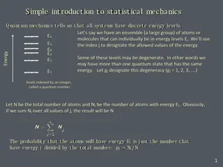
Linearized Boltzmann Equation in Statistical Mechanics

This lecture delves into the linearized Boltzmann equation and its applications in studying transport coefficients. The content covers the systematic approximation of transport coefficients, impact parameters of collisions, and the detailed solution for a dilute gas system. It explores the notation of the textbook, collision cross-sections, and the near-equilibrium assumptions. The discussion extends to the linearized Boltzmann equation for normal and tracer particles in the context of statistical mechanics.

• Statistical Mechanics
• Transport Coefficients
• Boltzmann Equation
• Linearization
• Dilute Gas

schrier_m Follow

Uploaded on Sep 25, 2024 | 0 Views

Download Presentation

Please find below an Image/Link to download the presentation.

The content on the website is provided AS IS for your information and personal use only. It may not be sold, licensed, or shared on other websites without obtaining consent from the author. Download presentation by click this link. If you encounter any issues during the download, it is possible that the publisher has removed the file from their server.

Presentation Transcript

1. PHY 770 -- Statistical Mechanics 12:00* - 1:45 PM TR Olin 107 Instructor: Natalie Holzwarth (Olin 300) Course Webpage: http://www.wfu.edu/~natalie/s14phy770 Lecture 22 Chap. 9 Transport coefficients Linearized Bolzmann equation Systematic approximation of the transport coefficients *Partial make-up lecture -- early start time 4/15/2014 PHY 770 Spring 2014 -- Lecture 22 1

2. Signup schedule for presentations available this afternoon. Please list the title of your presentation when you sign up. 4/15/2014 PHY 770 Spring 2014 -- Lecture 22 2

3. 4/15/2014 PHY 770 Spring 2014 -- Lecture 22 3

4. 4/15/2014 PHY 770 Spring 2014 -- Lecture 22 4

5. The Boltzmann equation: F f t + + = v ( , , ) r v f t r v t m coll With: f t = col l d d ( ) ( ) ( t f ) ( ) ( t f ) 3 v v , ', r v r v r v r v , ' , , , , , CM d d v f t f t 2 2 2 2 C M C M 4/15/2014 PHY 770 Spring 2014 -- Lecture 22 5

6. The Boltzmann equation: In the notation of your textbook: f t f = v ( ) ( ) , , r v , , r p t f t ( ) ( ) ( t f ) ( ) ( f ) 3 , ', r p r p r p r p ( , ) b g , ', , , , , d d p g f t f t t 2 2 2 CM cm coll where where impact parameter v of collisi on b g 2 Detailed solution for a dilute gas of N identical particles of mass m in volume V in absence of external force (F=0). In order to help the analysis, we will imagine that the particles are normal with label N and the particles are tracers with label T . The density of particles is denoted n0=N/V. 4/15/2014 PHY 770 Spring 2014 -- Lecture 22 6

7. The Boltzmann equation approximation by linearization Assume that the system is near equilibrium and define: = + r p p r p ( ) ( ) ( ) ( ) 0 , , 1 , , f t f h t 3/2 n ( ) p ( ) p ( ) p 2 = = = 0 0 0 /(2 ) p m In our case, 0 f f f e N T 2 2 m Define the possible collision cross sections for { , , , } for , : , cm a b g b c d = { , } , a b c d TT TN TN N N T = ( , ) 0 : , : , : : NN NN TT T N T , : , a b c d otherwise Abbrevi h ate: ( , r p ', ) t h for a=N or T. 1, 1 a a 4/15/2014 PHY 770 Spring 2014 -- Lecture 22 7

8. Linearized Boltzmann equation for normal and tracer particles 1 f + = v ( , r p , ) t h 1 1 r N t t , coll N 1 f + = v ( , r p , ) t h 1 1 r T t t , coll T 1 f ( ) d g , : , a b c d + 3 0 p ( ) d p f h h h h 2 2 1', 2', 1, 2, a b N c t , , a b c , coll N 1 f p ( ) d g , : , a b c d + 3 0 ( ) d p f h h h h 2 2 1', 2', 1, 2, a b T c t , , b c a , coll T 4/15/2014 PHY 770 Spring 2014 -- Lecture 22 8

9. Linearized Boltzmann equation for normal and tracer particles It is convenient to define the sum and difference distributions: and N T h h h h f t t + = + + h h N T 1 + + + + = v ( , r p C ( , r p , ) t , ) t h h 1 1 1 1 r + , coll 1 f v ( , r p C ( , r p , ) t , ) h h t 1 1 1 1 r t t , coll 1 f ( ) + + + + ( , ) b g f + 3 0 p 2 ( ) d p d g h h h h 2 2 1' 2 ' 1 2 t + , coll 1 f ( ) ( , ) b g f 3 0 p 2 ( ) d p d g h h 2 2 1 ' 1 t , coll 4/15/2014 PHY 770 Spring 2014 -- Lecture 22 9

10. Linearized Boltzmann equation for normal and tracer particles remarkable properties of collision operators Define the special inner prod uct: 3/2 2 1 ) ( /(2 ) p m 3 p p , ( ) d p e 1 1 1 2 m = ( ) + d g ( , ) b g f + 3 0 C ( , r p p , ) t 2 ( ) d p 2 1 1 2 1' 2' 1 2 r p Note that for an arbitrary function ( , , ): t 1 3 N V + = C , 1 4 2 m 2 ( ) d p d p 2 1 2 2 ( /(2 ))( + d g ( , b g + ) m p p 3 3 ) e 1 2 1' 2' 1 2 4/15/2014 PHY 770 Spring 2014 -- Lecture 22 10

11. Linearized Boltzmann equation for normal and tracer particles remarkable properties of collision operators -- continued Similar identity for difference collision opera ( , , ) d p t = Note that for an arbitrary function ( , tor ( ) d g ( , ) b g f 3 0 C r p p 2 ( ) 2 1 1 2 1' 1 r p , ): t 1 3 N V = C , 1 2 2 m 2 ( ) d p d p 2 1 2 2 ( /(2 ))( + d g ( , ) b g e ) m p p 3 3 1 2 1' 1 4/15/2014 PHY 770 Spring 2014 -- Lecture 22 11

12. Linearized Boltzmann equation for normal and tracer particles remarkable properties of collision operators continued Summary of results: 3 , 4 2 V m C N + = C 1 2 ( ) 2 1 2 2 ( /(2 ))( + d g ( , ) b g + ) m p p 3 3 d p d p e 1 2 1' 2' 1 2 + Eigenvalues o f are 0 1 2 p with 5 degenerate eigenvalues of 0 for 1, p , , ,2 p p x y z m 3 N V = C , 1 2 2 m 2 ( ) d p d p 2 1 2 2 ( /(2 ))( + d g ( , ) b g ) m p p 3 3 e 1 2 1' 1 C Eigenvalues of 0, with zero eigen vector 1 1 4/15/2014 PHY 770 Spring 2014 -- Lecture 22 12

13. Analysis of the diffusion coefficient r The difference in the tracer and normal particle densities at ( , ): t 3 = = 0 ( , ) r ( , ) r ( , ) r ( ) p ( , r p , ) t m t n t n t d p f h 1 1 1 N T h h h N T + = v ( , r p C ( , r p , ) t , ) t h h 1 1 1 1 r t 3 3 + = = 0 0 ( ) p v ( , r p ( ) p C ( , r p , ) t , ) t 0 d p f h d p f h 1 1 1 1 1 1 1 1 r t r ( , ) t m t 3 + = 0 D D J ( , ) r J ( , ) r ( ) p v ( , r p 0 where , ) t t t d p f h 1 1 1 1 r = D J ( , ) r ( , ) r Assume Fick's law: ( , ) t m t t D m t r r = 2 ( , ) r D m t r 4/15/2014 PHY 770 Spring 2014 -- Lecture 22 13

14. Analysis of the diffusion coefficient Need to solve the equation: + r p = v ( , r p C ( , r p , ) t , ) t h h 1 1 1 1 r t k r = i i t ( , )e k p Let C ( , , ) h t n 1 n ( Assume that ) = v k ( , ) k p ( , ) k p i i 1 1 n n n k | |is small (long wavelength cas + ( ) 1 ( , ) ( , ) n k + k p k p e ) k ( ) 0 ( ) 1 ( ) 2 + 2 .. .. k k n n n n ( ) 0 ( ) 2 + 2 ( , ) k p k p k p ( , )... k p k n n n ( ) 0 ( ) 0 = Assuming ( , )| ( , ) : ' n n nn ( ) 0 ( ) 0 ( ) 0 = ( , ) k p C ( , ) k p i 1 n n n ( ) 1 ( ) 0 ( ) 0 k = ( , ) k p v ( , ) , etc... p k 1 n n n 4/15/2014 PHY 770 Spring 2014 -- Lecture 22 14

15. Analysis of the diffusion coefficient -- continued = = ( , ) k p ( , ) k p Recall that has one zero eigenvalue and choose 1 0 n ( ) 0 ( ) 0 ( ) 0 = = ( , ) k p C ( , ) k p 0 i 0 0 1 0 3/2 1 m ( ) 1 ( ) 0 ( ) 0 k k 2 1 = = = /(2 ) p m 3 ( , ) k p v ( , ) k p p 0 d p e 0 1 1 1 n n 2 m ( ) ( ) ( ) 1 ( ) 2 ( ) 0 ( ) 1 ( ) 0 ( ) 1 ( ) 0 k k = + ( , ) k p v C v ( , ) k p i 0 1 0 1 0 1 0 n n 3/2 ( ) 1 1 k k 2 1 /(2 ) p m 3 p C p = d p e i 1 1 1 1 2 2 m m 3/2 ( ) 1 1 k k 2 1 = / (2 ) m p 3 p C p D d p e 1 1 1 1 2 2 m m 4/15/2014 PHY 770 Spring 2014 -- Lecture 22 15

16. Analysis of the diffusion coefficient -- continued 3/2 ( ) 1 1 k 2 1 = /(2 ) p m 3 p k C p D d p e 1 1 1 1 2 2 m m ( ) 1 k p = x C For convenience, let and def ine p x x 3 2 / 1 2 = /( 2 ) m p 3 D d pe p x x 2 2 m m Define Sonine polynomials (relatives of Laguerre polynomials) ( 1) ( ) ( 1)( l q l n l l = + + + + l n q n x ( 1) n q l S x )! ! 0 + + ( 1 ) q n = ' x n q n q Note that: ( ) x S ( ) x dxe S , n n ! n 0 2 p m = n q Expand: p d S x x n 2 = 0 n 4/15/2014 PHY 770 Spring 2014 -- Lecture 22 16

17. Analysis of the diffusion coefficient -- continued 3/2 3 2 2 m m 3/2 1 2 n m m = Evaluation of coefficient d 1 2 = /(2 ) p m D d pe p x x 2 p m = n q Expand: p d S x x n 2 = 0 n 2 1 p m 2 = = /(2 ) p m 3 2 n D d d pe p S d 3/2 0 n x 2 2 m 0 : 0 ( ) 1 p p = C C p p x x x x = 2 p m p n C p d S p 3/2 x n x 2 = 0 n 3/2 2 2 p m p m 2 p /(2 ) p m 3 ' n n C d pe p S p d S 3/2 3 / 2 x x n 2 2 2 m = 0 n 3 /2 2 p m 2 = /(2 ) p m 3 2 ' n d pe p S 3 / 2 x 2 2 m 4/15/2014 PHY 770 Spring 2014 -- Lecture 22 17

18. Analysis of the diffusion coefficient -- continued Evalua tion of coefficient : d 0 3/2 2 2 p m p m 2 p /(2 ) p m 3 ' n n C d pe p S p d S 3/2 3/2 x x n 2 2 2 m = 0 n 3/2 2 p m 2 = /(2 ) p m 3 2 ' n d pe p S 3/2 x 2 2 m m = D d n n , 0 n n = 0 n 3/2 2 2 p m p m 2 p /(2 ) p m 3 ' n n C w here D d pe p S p S n 3/2 3/2 n x x 2 2 2 m 4/15/2014 PHY 770 Spring 2014 -- Lecture 22 18

19. Analysis of the diffusion coefficient -- continued + Approximation of equation by trunction to m D d = 1: n n ,0 n n 0 n 1 ( ) 1 = lim D D 2 00 = Lowest order: 0 3/2 2 p = /(2 ) p m 3 C D d pe p p 00 x x 2 m Evaluation for the case of scattering from a hard sphere of radius : a 3/2 2 3 kT 2 p = = /(2 ) p m 3 C D d pe p p 00 x x 2 2 32 m n a m 0 3 1 kT = D 2 32 n a m 0 4/15/2014 PHY 770 Spring 2014 -- Lecture 22 19

20. Analysis of Viscosity and Thermal Conductivity For these transport coeffients, we need to evaluate the total scattering operator. Thermal conductivity: K = 3/2 ) ( ) 2 2 5 2 5 2 n m k p m p m 1 2 + 3 /(2 ) p m C 0 d pe p 1 x 2 2 2 2 m 3/2 ( ) ( n m 1 2 + = 3 /(2 ) p m C Shear viscosit y: 0 d pe p p p p 1 x y x y 2 2 m Previously, we have shown: 3 N V + = C , 1 4 2 m 2 ( ) 2 1 2 2 ( /(2 ))( + d g ( , ) b + ) m p p 3 3 d p d p g e 1 2 1' 2' 1 2 + C Eigenvalues of are 0 1 2 p with 5 degenerate eigenvalues of 0 for 1, p , x , ,2 p p y z m 4/15/2014 PHY 770 Spring 2014 -- Lecture 22 20

21. Analysis of viscosity and thermal conductivity -- continued Need to solve the equation: + r p + + + = v ( , r p C ( , r p , ) t , ) t h h 1 1 1 1 r t + + k r = i i t ( , )e k p Le t ( , , ) t h n 1 n ( For this case, we are interest i = C ) + + + = C v k ( , ) k p ( , ) k p i i 1 1 n n n ed in solutions near =0; the 5 zero eigenstates k + 0 are: 1 2 3 3 2 = = = = = + 2 1 p p p p 1 2 3 4 5 x y z 2 m m m m 4/15/2014 PHY 770 Spring 2014 -- Lecture 22 21

22. Analysis of viscosity and thermal conductivity -- continued ( Assume that ) + + + = C v k ( , ) k p ( , ) k p i i 1 1 n n n k | |is small (long wavelength case) + k ( ) 0 ( ) 1 ( ) 2 + 2 . ... k k n n n n ( ) 0 ( ) 1 ( ) 1 + + + + + + 2 ( , ) k p ( , ) k p ( , ) k p ( , )... p k k k n n n n ( ) 0 ( ) 0 + + = ( , k p ( , ) k p It is convenient to construct functions so t hat )| : ' n n nn ( ) 0 = For the 5 states: 0 n ( ) 1 = By construction: 0 n ( ) 2 = 2 k n n 4/15/2014 PHY 770 Spring 2014 -- Lecture 22 22

23. Analysis of viscosity and thermal conductivity -- continued Following Eqs. 9.121-9.124 of your text and using: = = 2 3 3 2 = = = + 2 1 p p p p 1 2 3 4 5 x y z 2 m m m m 1 3 5 2 5 + = + + (0) 1 1 5 2 2 1 3 5 2 5 + = + (0) 2 1 5 2 2 + + = = 0) 3 ( (0) 4 3 4 2 5 3 5 + = + ( 5 0) 1 5 4/15/2014 PHY 770 Spring 2014 -- Lecture 22 23

24. Analysis of thermal conductivity -- continued Following Sect. 9.7.3 of your text, we can write the thermal conductivity coefficient: 3/2 m 2 2 5 2 n m k p m p m 2 = 3 /(2 ) 2 p m n 0 K a d pe p S 3/2 n x 2 2 2 2 m = 0 n 5 2 5 2 n m k = = where 0 a M a n n 1 ,1 n n = 0 n 3/2 2 2 p m p m 2/( + p 2 ) m p 3 ' n n C and M d pe p S p S n n 3 /2 3/ 2 x x 2 2 2 m Estimate for hard sphere scattering of radius a 75 256 k a kT m = K 2 4/15/2014 PHY 770 Spring 2014 -- Lecture 22 24

25. Analysis of shear viscosity-- continued Following Sect. 9.7.4 of your text, we can write the shear viscosity coefficient: 3/2 2 n m p m 2 = 3 /(2 ) 2 2 y p m n 0 b d pe p p S 5/2 n x 2 2 2 m = 0 n 2 n m = = where 0 b n n n N b 0 ,0 n 2 = 0 n 3/2 2 2 p m p m 2 + p /(2 ) p m 3 ' n n C and N d pe p p S p p S n n 5/2 5/2 x y x y 2 2 2 m Estimate for hard sphere scattering of radius a 5 mkT = 2 64 a 4/15/2014 PHY 770 Spring 2014 -- Lecture 22 25