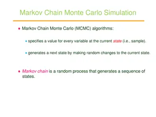
Understanding MCMC Sampling Methods in Bayesian Estimation

Bayesian statistical modeling often relies on Markov chain Monte Carlo (MCMC) methods for estimating parameters. This involves sampling from full conditional distributions, which can be complex when software limitations arise. In such cases, the need to implement custom MCMC samplers may arise, requiring a deeper understanding of the underlying concepts and techniques. This process involves selecting and executing MCMC samplers to improve estimation accuracy and efficiency.

• Bayesian estimation
• MCMC methods
• Markov chain Monte Carlo
• Statistical modeling
• Sampling techniques

rier780 Follow

Uploaded on Sep 26, 2024 | 0 Views

Download Presentation

Please find below an Image/Link to download the presentation.

The content on the website is provided AS IS for your information and personal use only. It may not be sold, licensed, or shared on other websites without obtaining consent from the author. Download presentation by click this link. If you encounter any issues during the download, it is possible that the publisher has removed the file from their server.

Presentation Transcript

1. MCMC Sampling: Creating a Generic Sampler & Comparison of MCMC Algorithms Earl Duncan Bayesian Research and Applications Group (BRAG) 7 Nov 2019

2. Introduction Part 1: Generic Sampler Part 2: Comparing Samplers Results Introduction: The main task of statistical modelling is estimating the unknown parameters. In Bayesian methodology, Markov chain Monte Carlo (MCMC) methods are one of the most popular classes of estimation methods. o Make use of the full conditional distributions, or simply full conditionals (FCs). o The techniques available depend on the properties of the FCs. Most of the time, we use software to do the heavy lifting for us: o Automatically deriving the FCs from the (marginal) priors and likelihood; o Determining which MCMC methods are appropriate/optimal for a given FC; o Actually implementing the MCMC methods; o Automatically tuning MCMC sampler specific tuning parameters; and o Possibly more (guessing an appropriate burn-in, initial values, etc.) Common software includes WinBUGS/OpenBUGS, JAGS, stan, CARBayes (R package) Software in development: greta (Nick Golding, BotB 2017) Earl Duncan BRAG 7 Nov 2019 1

3. Introduction Part 1: Generic Sampler Part 2: Comparing Samplers Results Motivation: Sometimes the available software may be too restrictive for your use case. E.g. o Does not allow certain distributions or link functions (if not built-in , often there are hacks to introduce custom-defined distributions and link functions). o Does not allow certain models (e.g. JAGS prohibits cyclic graphs, so no CAR models). o Does not operate in certain environment (e.g. supercomputer nodes). o Does not handle high dimensions. o Is not efficient. In these cases, you may need to implement the models and estimation yourself. This is no easy feat! o All that heavy-lifting done by software (see slide 1) now needs to be done by you. o Deriving the FCs generally isn t too difficult (see my BRAG talk from 18 Aug 2016 for a guide). o In this presentation, I focus on the task of choosing and implementing MCMC sampler(s) Earl Duncan BRAG 7 Nov 2019 2

4. Introduction Part 1: Generic Sampler Part 2: Comparing Samplers Results Monte Carlo to MCMC: Consider the FC for some parameter ? ? ? ?,?,? Gamma ?;? + ??,? + ? ?=1 where ? = (?1, ,??) is observed data. For fixed values of ? and ?, we can use Monte Carlo methods to repeatedly sample from this distribution (or a transformation of it) to obtain an i.i.d. sample for ?. In R, we can generate such random variates for most well-known distributions using rgamma, rnorm, rpois, rexp, etc. Use Monte Carlo sampling Have a look at the help files to see what technique. E.g. ?rexp Earl Duncan BRAG 7 Nov 2019 3

5. Introduction Part 1: Generic Sampler Part 2: Comparing Samplers Results Monte Carlo to MCMC (cont.): ? ? ?,?,? Gamma ?;? + ??,? + ? ?=1 But what if ? and ? are also unknown parameters? We now have 3 FCs, each dependent on the other two parameters. We need to update our estimates of the two input parameters each time we take sample (each iteration). But generated sample will no longer be i.i.d. However, once convergence is reached, samples should be mostly independent. Earl Duncan BRAG 7 Nov 2019 4

6. Introduction Part 1: Generic Sampler Part 2: Comparing Samplers Results Historic overview of MCMC Samplers: Extensions: Metropolis 1953 Metropolis-Hastings (MH) 1970 Gibbs 1984 (Improved efficiency?) 1990 Hamiltonian Monte Carlo (HMC) No U-turn sampler (NUTS) extension 2014 1987 Adaptive rejection sampling (ARS)* 1992 ARMS 1995 2010 CCARS Slice sampling (SS) 1997 2003 Multivariate SS & many extensions * Original version used derivatives. A derivative-free version was published later that same year. WinBUGS uses the derivative-free version. My results are based on the gradient-based version. Earl Duncan BRAG 7 Nov 2019 5

7. Introduction Part 1: Generic Sampler Part 2: Comparing Samplers Results Note on WinBUGS: Software may implement a single sampler, or choose from a set of samplers. E.g. WinBUGS chooses a sampler as by a process of elimination: Source: the WinBUGS manual Earl Duncan BRAG 7 Nov 2019 6

8. Introduction Part 1: Generic Sampler Part 2: Comparing Samplers Results Part 1: Creating a Generic Sampler (using potentially different MCMC algorithms for each FC) Earl Duncan BRAG 7 Nov 2019 7

9. Introduction Part 1: Generic Sampler Part 2: Comparing Samplers Results Goal: Develop a framework (R package) for implementing any arbitrary model which gives the user complete flexibility over what sampler is used for any set of FCs. User must first determine each FC (or joint distribution) and decide which sampler to use. The FC and MCMC sampler specific functions (see slide 11) are passed to a specialised sampling function which calls the necessary subroutines. A posterior sample is obtained by looping over iterations. Earl Duncan BRAG 7 Nov 2019 8

10. Introduction Part 1: Generic Sampler Part 2: Comparing Samplers Results Work flow: 1. Define the model (likelihood and prior specification) (Currently working with single kernel densities see slide 16) Derive the FCs Decide which sampler to use for each FC. As a rough guide: 2. 3. Global requirements: MH algorithm requires a suitable proposal density. Gradient-based ARS algorithm requires the target density be log-concave. HMC will work for discrete distributions if pmf can be evaluated on a continuous domain e.g. by using gamma function instead of factorial (see next slide) Earl Duncan BRAG 7 Nov 2019 9

11. Introduction Part 1: Generic Sampler Part 2: Comparing Samplers Results Aside: using HMC for discrete distributions: If the pmf can be rewritten to return non-zero density on a continuous support, HMC should be viable. E.g. for the Poisson distribution, you just need to replace the factorial function ?! with gamma functions (? + 1). This works for Poisson, Bernoulli, binomial, negative binomial, multinomial, and geometric. It does not work for the categorical distribution. Earl Duncan BRAG 7 Nov 2019 10

12. Introduction Part 1: Generic Sampler Part 2: Comparing Samplers Results Work flow (cont.): 4. Derive/define any MCMC sampler specific functions. (ERS is a brute force Monte Carlo envelope-rejection sampler, included for validation) Note: ? is the full conditional; ? is a proposal/envelope density; the potential energy function is ? ? = log?(?) and its gradient is ?? ? ??log?(?), so these can be ? ??log?(?). ??= replaced by calls to functions for log?(?) and its gradient ? = Earl Duncan BRAG 7 Nov 2019 11

13. Introduction Part 1: Generic Sampler Part 2: Comparing Samplers Results Work flow (cont.): 5. Convert to R code functions. E.g. for parameter ? ? ?;?,?2 Earl Duncan BRAG 7 Nov 2019 12

14. Introduction Part 1: Generic Sampler Part 2: Comparing Samplers Results Work flow (cont.): 6. Pass these functions to the respective sampler function and loop to obtain a sample. E.g. for a sample using SS: SS sampler function (log) full conditional from previous slide Earl Duncan BRAG 7 Nov 2019 13

15. Introduction Part 1: Generic Sampler Part 2: Comparing Samplers Results Part 2: Comparison of MCMC Algorithms Earl Duncan BRAG 7 Nov 2019 14

16. Introduction Part 1: Generic Sampler Part 2: Comparing Samplers Results Goal: How do these MCMC samplers perform for: multi-modal distributions? truncated distributions? discrete distributions? multivariate distributions? non-scalar parameters? 1 multivariate distribution vs ? univariate distributions? autocorrelated parameters? 1 multivariate distribution vs ? univariate distributions? (WIP no results yet) Earl Duncan BRAG 7 Nov 2019 15

17. Introduction Part 1: Generic Sampler Part 2: Comparing Samplers Results Test samplers across different models: Very simple models! No priors (1 FC; 1 (possibly non-scalar) unknown parameter) No observed data (but all input parameters assumed known) No autocorrelation ? = 5,? = 5 Earl Duncan BRAG 7 Nov 2019 16

18. Introduction Part 1: Generic Sampler Part 2: Comparing Samplers Results Results: Model 1: Gaussian density Earl Duncan BRAG 7 Nov 2019 17

19. Introduction Part 1: Generic Sampler Part 2: Comparing Samplers Results Results: Model 2: bimodal density Note: Generally ARS does not work for models like this which are not log-concave. However, with a bit of luck, the code may execute without run-time errors, but the results are likely to be very poor around convex portions of the distribution. Derivative-free versions of ARS or other extensions are required for good results. Earl Duncan BRAG 7 Nov 2019 18

20. Introduction Part 1: Generic Sampler Part 2: Comparing Samplers Results Results: Model 3: multi-modal density Looks like each algorithm struggles with this one, either over- or under-sampling different regions of high density (or missing modes completely). Earl Duncan BRAG 7 Nov 2019 19

21. Introduction Part 1: Generic Sampler Part 2: Comparing Samplers Results Results: Model 4: truncated density Note: increasing the mass and decreasing the step size tuning parameters (HMC) can help for truncated distributions (step sizeshould be auto-tuned during burn-in). Otherwise Earl Duncan BRAG 7 Nov 2019 20

22. Introduction Part 1: Generic Sampler Part 2: Comparing Samplers Results Results: Model 5: discrete distribution Recall HMC can be used for discrete distributions provided they can be evaluated on a continuous domain (see slide 10 for details). Earl Duncan BRAG 7 Nov 2019 21

23. Introduction Part 1: Generic Sampler Part 2: Comparing Samplers Results Results: Model 6: density with a very narrow domain ERS struggles unless the envelope (proposal) distribution is very close to the true posterior. Earl Duncan BRAG 7 Nov 2019 22

24. Introduction Part 1: Generic Sampler Part 2: Comparing Samplers Results Results: Model 7a: vector-valued parameter (univariate FCs) Earl Duncan BRAG 7 Nov 2019 23

25. Introduction Part 1: Generic Sampler Part 2: Comparing Samplers Results Results: Model 7b: vector-valued parameter (1 multivariate FC, but marginal posteriors plotted) Only MH and HMC attempted for multivariate FC distributions (see slide 9). Earl Duncan BRAG 7 Nov 2019 24

26. Introduction Part 1: Generic Sampler Part 2: Comparing Samplers Results Results: Model 8: multivariate FC Only MH and HMC attempted for multivariate FC distributions (see slide 9). Earl Duncan BRAG 7 Nov 2019 25

27. Introduction Part 1: Generic Sampler Part 2: Comparing Samplers Results Computation time: All models Model 7 (vector-valued parameter) may be faster to treat parameter as multivariate (7b) rather than iid univariate (7a). But SS and ARS really only work well when univariate. For larger dimensions, it is probably more efficient to do multivariate (see slide 28). Earl Duncan BRAG 7 Nov 2019 26

28. Introduction Part 1: Generic Sampler Part 2: Comparing Samplers Results Computation time: Model 7a variants ?: Burnin: Sample size: 10 2000 5000 20 2000 5000 5 4000 10000 5 2000 5000 Earl Duncan BRAG 7 Nov 2019 27

29. Introduction Part 1: Generic Sampler Part 2: Comparing Samplers Results Computation time: Model 7b variants ? ?: 5 5 5 10 20 5 25 5 5 50 10 5 15 5 Multivariate version scales well with data sample size, ?, as expected. Earl Duncan BRAG 7 Nov 2019 28

30. Introduction Part 1: Generic Sampler Part 2: Comparing Samplers Results Computation time: Model 8 variants ?: 10 20 30 2 Computation time in adjusted model has been inflated for rejection rate. Earl Duncan BRAG 7 Nov 2019 29

31. Key references: Duane, S., A.D. Kennedy, B. J. Pendleton, and D. Roweth. 1987. Hybrid Monte Carlo. Physics Letters B195 (2): 216-222. DOI: 10.1016/0370- 2693(87)91197-x. Gilks, W. R. and P. Wild. 1992. Adaptive rejection sampling for Gibbs sampling. Applied Statistics41 (2): 337-348. DOI: 10.2307/2347565. Gilks, W. R. 1992 Derivative-free adaptive rejection sampling for Gibbs sampling . In Bayesian Statistics 4, edited by J. Bernardo, J. Berger, A. P. Dawid, and A. F. M. Smith. Oxford University Press. Hastings, W. K. 1970. Monte Carlo sampling methods using Markov chains and their applications. Biometrika57 (1): 97-109. DOI: 10.2307/2334940. Neal, R. M. 1997. Markov chain Monte Carlo methods based on slicing the density function. Technical report no. 9722, Department of Statistics, University of Toronto. Available at www.cs.toronto.edu/~ radford/slice.abstract.html. 1987 1992 1970 1997 Contact: earl.duncan@qut.edu.au https://bragqut.wordpress.com/people/earl-duncan/ Earl Duncan BRAG 7 Nov 2019 30