Quantum Deep Learning: Challenges and Opportunities in Artificial Intelligence
Quantum deep learning explores the potential of using quantum computing to address challenges in artificial intelligence, focusing on learning complex representations for tough AI problems. The quest is to automatically learn representations at both low and high levels, leveraging terabytes of web data for training. Deep networks play a crucial role in understanding object recognition, with recent advancements showing significant improvements in error rates on various tasks. The primary challenges include learning complex representations efficiently, computing true gradients, and reducing training time, prompting the exploration of quantum computing as a possible solution.

Download Presentation

Please find below an Image/Link to download the presentation.
The content on the website is provided AS IS for your information and personal use only. It may not be sold, licensed, or shared on other websites without obtaining consent from the author. Download presentation by click this link. If you encounter any issues during the download, it is possible that the publisher has removed the file from their server.
E N D
Presentation Transcript
Quantum Deep Learning Nathan Wiebe, Ashish Kapoor and Krysta Svore Microsoft Research ASCR Workshop Washington DC 1412.3489
The problem in artificial intelligence How do we make computers that see, listen, and understand? Goal: Learn complex representations for tough AI problems Challenges and Opportunities: Terabytes of (unlabeled) web data, not just megabytes of limited data No silver bullet approach to learning Good new representations are introduced only every 5-10 years Can we automatically learn representations at low and high levels? Does quantum offer new representations? New training methods?
Deep networks learn complex representations object recognition Desired outputs ?1 ?2 ?? ?? High-level features object properties ?1 1 ?2 2 ?? ? ?? ? 1 1 Mid-level features textures ?1 1 ?2 2 ?? ? ?? ? 1 1 Difficult to specify exactly Low-level features edges ?1 1 ?2 2 ?? ? ?? ? 1 1 Deep networks learn these from data without explicit labels Input pixels ?1 ?2 ?? ?? 1 Analogy: layers of visual processing in the brain
Why is deep learning so important? Deep learning has resulted in significant improvements in last 2-3 years 30% relative reduction in error rate on many vision and speech tasks Approaching human performance in limited cases (e.g., matching 2 faces) New classical deep learning methods already used in: Language models for speech Web query understanding models Machine translation Deep image understanding (image to text representation)
Primary challenges in learning Desire: learn a complex representation (e.g., full Boltzmann machine) Intractable to learn fully connected graph poorer representation Pretrain layers? Learn simpler graph with faster train time? Can we learn a more complex representation on a quantum computer? Desire: efficient computation of true gradient Intractable to learn actual objective poorer representation Approximate the gradient? Can we learn the actual objective (true gradient) on a quantum computer? Desire: training time close to linear in number of training examples Slow training time slower speed of innovation Build a big hammer? Look for algorithmic shortcuts? training on a quantum computer? Can we exponentially speedup model
Restricted Boltzmann Machine Energy of system is given by an Ising model on a bipartite graph. Hidden units 0 1 1 Visible units 0 1 0 1 Data
Restricted Boltzmann Machine Energy of system is given by an Ising model on a bipartite graph. Hidden units 0 1 1 Energy penalty applied if connected bits have the same value. Probability is given by Gibbs distribution over states. Visible units 0 1 0 1 Choose edges weights to maximize P(data). Data
Deep Restricted Boltzmann Machine 1 1 Hidden units 0 0 1 1 Higher-level features 0 1 0 1 Features Data
Key steps Classically compute a mean-field approximation to Gibbs state Prepare the mean-field state on a quantum computer Refine the mean-field state into the Gibbs state by using measurement and post selection Measure the state and infer the likelihood gradient from the measurement statistic
How does the refining work? Uses HHL-style state preparation ? ?(?, ) ???????? ?, ? ?(?, ) ???????? ?, ?, ?(?, ) ?, 1 + 1 0 . If 1 measured then you prepare a coherent analog of Gibbs. Amplitude amplification, amplitude estimation, other optimizations are also used.
Performance of method ? = number of edges in whole graph. = number of layers in deep Restricted Boltzmann Machine ? = maximum ratio between MF and Gibbs probabilities
Conclusions We provide new quantum algorithms for learning using deep Boltzmann machines. Key contribution is state preparation technique. Our algorithms Train without the contrastive divergence approximation Avoid greedy layer-by-layer training Generalize to full unrestricted Boltzmann machines May lead to much smaller models or more accurate models Offers polynomial speedups for dRBMs
Open questions How can we take advantage of the quantumness of Hamiltonians for learning? Does quantum give us the ability to ask entirely new questions? How can we approach the input/output problem in quantum algorithms? We give one algorithm that avoids QRAM What other methods are there to deal with large data?
Preparation of Gibbs state If we can prepare the state ?, ?(?, ) then the resulting state is proportional to ?(?, ) Add a quantum register to compute ?(?, ) Compute the likelihood ratio in superposition to efficiently prepare: ?(?, ) ? and multiply it by If 1 is measured on last qubit then the resultant state is the Gibbs state The success probability can be boosted by using amplitude amplification ? 1 ????????= ???? ?