Understanding 2D Viewing Transformations and Windowing Concepts

Exploring two-dimensional transformations, homogeneous coordinate systems, matrix formulation, and concatenation of transformations. Concepts like windowing, window-to-viewport transformation, viewing transformation, and the 2D viewing pipeline are discussed with relevant images and explanations.

Download Presentation

Please find below an Image/Link to download the presentation.
The content on the website is provided AS IS for your information and personal use only. It may not be sold, licensed, or shared on other websites without obtaining consent from the author. Download presentation by click this link. If you encounter any issues during the download, it is possible that the publisher has removed the file from their server.
E N D
Presentation Transcript
MODULE III Two dimensional transformations. Homogeneous coordinate systems matrix formulation and concatenation of transformations. Windowing concepts Window to Viewport Transformation- Two dimensional clipping-Line clipping Cohen Sutherland, Midpoint Subdivision algorithm
Windowing Concepts A world co-ordinate area selected for display is called a window An area on a display device to which a window is mapped is called a viewport. Window defines what is to be displayed. Viewport defines where it is to be displayed. Windows & viewports are rectangles in standard position,with rectangle edges parallel to the co-ordinate axes.
Viewing Transformation The mapping of a part of a world-coordinate scene to device coordinates is referred to as a viewing transformation. Sometimes the two-dimensional viewing transformation is simply referred to as the window-to-viewport transformation or the windowing transformation.
Viewing Transformation the term window refers to an area of a world co-ordinate scene that has been selected for display picture that is selected for viewing
2D viewing Pipeline Some graphics packages that provide window and viewport operations allow only standard rectangles, but a more general approach is to allow the rectangular window to have any orientation. In this case, we carry out the viewing transformation in several steps, as indicated in this figure
Viewing transformation pipeline (1) First, we construct the scene in world coordinates using the output primitives and attributes Next. To obtain a particular orientation for the window, we can set up a two-dimensional viewing-coordinate system in the world-coordinate plane, and define a window in the viewing-coordinate system. The viewing coordinate reference frame is used to provide a method for setting up arbitrary orientations for rectangular windows. Once the viewing reference frame is established, we can transform descriptions in world coordinates to viewing coordinates.
Viewing transformation pipeline (1) We then define a viewport in normalized coordinates (in the range from 0 to 1 ) and map the viewing-coordinate description of the scene to normalized coordinates. At the final step, all parts of the picture that lie outside the viewport are clipped, and the contents of the viewport are transferred to device coordinates.
Zooming and Panning effects By changing the position of the viewport, we can view objects at different positions on the display area of an output device. Also, by varying the size of viewports, we can change the size and proportions of displayed objects. We achieve zooming effects by successively mapping different-sized windows on a fixed-size viewport. As the windows are made smaller, we zoom in on some part of a scene to view details that are not shown with larger windows. Similarly, more overview is obtained by zooming out from a section of a scene with successively larger windows. Panning effects are produced by moving a fixed-sizewindow across the various objects in a scene
VIEWING COORDINATE REFERENCE FRAME This coordinate system provides the reference frame for specifying the world coordinate window
VIEWING COORDINATE REFERENCE FRAME We set up the viewing coordinate system using the following procedures: First, a viewing-coordinate origin is selected at some world position: po = (x0, y0). Then we need to establish the orientation, or rotation, of this reference frame. One way to do this is to specify a world vector v that defines the viewing yv, direction. Vector v is called the view up vector.
VIEWING COORDINATE REFERENCE FRAME Given V, we can calculate the components of unit vectors v = (vx, vy) and U = (ux, uy) for the viewing yv, and xv, axes, respectively. These unit vectors are used to form the first and second rows of the rotation matrix r that aligns the viewing xv yv axes with the world xw yw axes. We obtain the matrix for converting world coordinate positions to viewing Coordinates as a two-step composite transformation: First, we translate the viewing origin to the world origin, then we rotate to align the two coordinate reference frames.
VIEWING COORDINATE REFERENCE FRAME the composite two-dimensional transformation to convert world coordinates to viewing coordinate is Where T is the translation matrix that takes the viewing origin point po to the world origin, and R is the rotation matrix that aligns the axes of the two reference frames.
Clipping Operations Procedure that identifies those portions of a picture that are either inside or outside of a specified region of space Region against which an object is to be clipped is called a clip window
Point Clipping The Clip window is a rectangle to the standard position, we save a point P=(x,y) for display if the following inequalities are satisfied: xwmin<=x<=xwmax ywmin<=y<=ywmax Where the edges of the clip window (xwmin ,xwmax) and (ywmin, ywmax), can be either the coordinate window boundaries. If any one of these four inequalities is not satisfied , the point is clipped. 18
ywmax P( x, y) ywmin xwmin xwmax Figure: Point Clipping 19
Line Clipping Line that do not intersect the clipping window are either completely inside the window or completely outside the window. In the case of line clipping , three different cases are possible. p3 p4 p9 ywmax p2 p10 p1 p6 Window p5 p7 ywmin p8 xwmax 20 xwmin
Different cases for Line Clipping 1. Both endpoints of the line lie with in the clipping area. This means that the line is included completely in the clipping area, so that the whole line must be drawn. B B A A Clip rectangle 21
2. One end point of the line lies with in the other outside the clipping area. It is necessary to determine the intersection point of the line with the bounding rectangle of the clipping area. Only a part of the line should be drawn. D D D B B C C C A A Clip rectangle 22
3. Both end points are located outside the clipping area and the line do not intersect the clipping area. In the case , the line lies completely outside the clipping area and can be neglected for the scene. 4. Both endpoints are located outside the clipping area and the line intersect the clipping area. The two intersection points of the line with the clipping are must be determined. Only the part of the line between these two intersection points should be drawn. D E D D B H C B C F H' J A H' G A J G Clip rectangle G I I 23
This algorithm divides a 2D space into 9 parts, of which only the middle part is visible. This method is used: To save a line segment. To discard line segment To divide the line according to window co- ordinate. Cohen Sutherland performs line clipping in two phases: Phase1: Find visibility of line. Phase2: clip the line falling in category 3 (candidate for Clipping). i. ii. iii. 24
COHEN-SUTHERLAND LINE CLIPPING ALGORITHM This is one of the oldest and most popular line-clipping procedures. The method speeds up the processing of line segments by performing initial tests that reduce the number of intersections that must be calculated. Every line endpoint in a picture is assigned a four digit binary code called a region code that identifies the location of the point relative to the boundaries of the clipping rectangle.
Binary region codes assigned to line end points according to relative position with respect to the clipping rectangle. Region are set up in reference as shown in figure: LEFT RIGHT y 1010 1001 1000 ywmax TOP window 0001 0000 0010 ywmin BOTTOM 0101 0100 0110 x xwmin xwmax Figure :Bit Code for Cohen- Sutherland clipping 26
Each bit position in region code is used to indicate one of four relative coordinate positions of points with respect to clip window: to the left, right, top or bottom. By numbering the bit positions in the region code as 1 through 4 from right to left, the coordinate regions are corrected with bit positions as bit 1: left bit 2: right bit 3: below bit4: above A value of 1 in any bit position indicates that the point is in that relative position. Otherwise the bit position is set to 0. If a point is within the clipping rectangle the region code is 0000. A point that is below and to the left of the rectangle has a region code of 0101.
region-code bit values can be determined with following two steps. (1) Calculate differences between endpoint coordinates and clipping boundaries. (2) Use the resultant sign bit of each difference calculation to set the corresponding value in the region code. bit 1 is the sign bit of x xwmin bit 2 is the sign bit of xwmax - x bit 3 is the sign bit of y ywmin bit 4 is the sign bit of ywmax - y.
Once we have established region codes for all line endpoints, we can quickly determine which lines are completely inside the clip window and which are clearly outside. Any lines that are completely contained within the window boundaries have a region code of 0000 for both endpoints, and we accept these lines. Any lines that have a 1 in the same bit position in the region codes for each endpoint are completely outside the clipping rectangle, and we reject these lines.
COHEN-SUTHERLAND LINE CLIPPING ALGORITHM Step 1 Compute the regioncodes for the two end points of the segment Step 2 Enter a loop, within the loop check to see if both the regioncodes are zero. Then enter the segment into the display file, exit the loop & return
COHEN-SUTHERLAND LINE CLIPPING ALGORITHM Step 3 If both the region codes are not zero then take Logical AND of both the regioncodes & check for non-zero result. If so , then reject the line, exit the loop & return. Step 4 If the result is 0, then subdivide the line segment from intersection point of line segment & clipping boundary. Step 5 Repeat steps (2), (3) & (4) for each segment.
Intersection points with a clipping boundary can be calculated using the slope-intercept form of the line equation. For a line with endpoint coordinates (x1,y1) and (x2,y2) the y coordinate of the intersection point with a vertical boundary can be calculated as y =y1 +m (x-x1) where x value is set either to xwmin or to xwmax and slope of line is calculated as m = (y2- y1) / (x2- x1) the x coordinate of the intersection point with a horizontal boundary can be calculated as x= x1 +( y- y1) / m with y set to either to ywmin or to ywmax.
Example: Starting with the bottom endpoint of the line from P1 to P2, we check P1 against the left, right, and bottom boundaries in turn and find that this point is below the clipping rectangle. We then find the intersection point P1 with the bottom boundary and discard the line section from P1 to P1 . The line now has been reduced to the section from P1 to P2
Since P2, is outside the clip window, we check this endpoint against the boundaries and find that it is to the left of the window. Intersection point P2 is calculated, but this point is above the window. So the final intersection calculation yields P2 , and the line from P1 to P2 is saved. This completes processing for this line Point P3 in the next line is to the left of the clipping rectangle, so we determine the intersection P3 , and eliminate the line section from P3 to P3 . By checking region codes for the line section from P3'to P4 we find that the remainder of the line is below the clip window and can be discarded also.
Mid point subdivision algorithm This method divide the line into three category: I. Category 1: Visible line II. Category 2: not visible line III. Category 3: candidate for Clipping. An alternative way to process a line in category 3 is based on binary search. The line is divided at its midpoints into two shorter line segments. Each line in a category three is divided again into shorter segments and categorized. This bisection and categorization process continue until each line segment that spans across a window boundary reaches a threshold for line size and all other segments are either in a category 1 (visible) or in category 2 (Not visible.) 35
Mid point subdivision algorithm An alternative way to process a line in category 3 is based on binary search. The line is divided at its midpoints into two shorter line segments. Each line in a category three is divided again into shorter segments and categorized. This bisection and categorization process continue until each line segment that spans across a window boundary reaches a threshold for line size and all other segments are either in a category 1 (visible) or in category 2 (Not visible.)
Mid-point subdivision algorithm The mid points coordinates are (x m , y m) of a line joining the points(X1,Y1)and (X2,Y2) are given by: X m= X1+X2/2 and Y M= Y1+Y2/2 Q I2 24 3 1 I1 6785 P Figure: illustrates how midpoint subdivision is used to zoom in onto the two Intersection points I1 and I2 with 10 bisection. 37
Comparison b/w Cohen-Sutherland and Mid-point subdivision clipping Algorithm Midpoint subdivision algorithm is a special case of Cohen-sutherland algorithm, where the intersection is not computed by equation solving. It is computed by a midpoint approximation method, which is suitable for hardware and it is very fast and efficient. The maximum time is consume in the clipping process is to do intersection calculation with the window boundaries. The Cohen-sutherland algorithm reduces these calculation by first discarding that lines those can be trivially accepted or rejected. 38


")
")