Understanding GraphPlan Algorithm for Efficient Planning

GraphPlan, introduced in 1995, revolutionized planning research by reducing the branching factor for search algorithms. By creating a planning graph and enabling solution extraction, GraphPlan inspired newer, more effective planning techniques. Layered plans and executing actions in sets play a key role in GraphPlan's approach to efficient planning.

Download Presentation

Please find below an Image/Link to download the presentation.
The content on the website is provided AS IS for your information and personal use only. It may not be sold, licensed, or shared on other websites without obtaining consent from the author. Download presentation by click this link. If you encounter any issues during the download, it is possible that the publisher has removed the file from their server.
E N D
Presentation Transcript
GraphPlan Alan Fern * * Based in part on slides by Daniel Weld and Jos Luis Ambite 1
GraphPlan http://www.cs.cmu.edu/~avrim/graphplan.html Many planning systems use ideas from Graphplan: IPP, STAN, SGP, Blackbox, Medic, FF, FastDownward History Before GraphPlan appeared in 1995, most planning researchers were working under the framework of plan-space search (we will not cover this topic) GraphPlan outperformed those prior planners by orders of magnitude GraphPlan started researchers thinking about fundamentally different frameworks Recent planning algorithms are much more effective than GraphPlan However, many have been influenced by GraphPlan 2
Big Picture A big source of inefficiency in search algorithms is the large branching factor GraphPlan reduces the branching factor by searching in a special data structure Phase 1 Create a Planning Graph built from initial state contains actions and propositions that are possibly reachable from initial state does not include unreachable actions or propositions Phase 2 - Solution Extraction Backward search for the solution in the planning graph backward from goal 3
Layered Plans Graphplan searches for layered plans (often called parallel plans) A layered plan is a sequence of sets of actions actions in the same set must be compatible a1 and a2 are compatible iff a1 does not delete preconditions or positive effects of a2 (and vice versa) all sequential orderings of compatible actions gives same result ? A B D C B C D A Layered Plan: (a two layer plan) move(B,TABLE,A) move(D,TABLE,C) move(A,B,TABLE) move(C,D,TABLE) ; 4
Executing a Layered Plans A set of actions is applicable in a state if all the actions are applicable. Executing an applicable set of actions yields a new state that results from executing each individual action (order does not matter) D C B A B C move(A,B,TABLE) move(C,D,TABLE) A B A D D C move(B,TABLE,A) move(D,TABLE,C) 5
Planning Graph A literal is just a positive or negative propositon A planning graph has a sequence of levels that correspond to time-steps in the plan: Each level contains a set of literals and a set of actions Literals are those that could possibly be true at the time step Actions are those that their preconditions could be satisfied at the time step. Idea: construct superset of literals that could be possibly achieved after an n-level layered plan Gives a compact (but approximate) representation of states that are reachable by n level plans 6
Planning Graph state-level 0: propositions true in s0 state-level n: literals that may possibly be true after some n level plan action-level n: actions that may possibly be applicable after some n level plan s0 sn an Sn+1 propositions actions 7
Planning Graph maintenance action (persistence actions) represents what happens if no action affects the literal include action with precondition c and effect c, for each literal c propositions actions 8
Graph expansion Initial proposition layer Just the propositions in the initial state Action layer n If all of an action s preconditions are in proposition layer n, then add action to layer n Proposition layer n+1 For each action at layer n (including persistence actions) Add all its effects (both positive and negative) at layer n+1 (Also allow propositions at layer n to persist to n+1) Propagate mutex information (we ll talk about this in a moment) 9
Example stack(A,B) precondition: holding(A), clear(B) effect: ~holding(A), ~clear(B), on(A,B), clear(B), handempty s0 a0 s1 holding(A) ~holding(A) holding(A) handempty stack(A,B) ~clear(B) on(A,B) clear(B) clear(B) 10
Example stack(A,B) precondition: holding(A), clear(B) effect: ~holding(A), ~clear(B), on(A,B), clear(B), handempty s0 a0 s1 holding(A) ~holding(A) holding(A) handempty stack(A,B) ~clear(B) on(A,B) clear(B) clear(B) Notice that not all literals in s1 can be made true simultaneously after 1 level: e.g. holding(A), ~holding(A) and on(A,B), clear(B) 11
Mutual Exclusion (Mutex) Mutex between pairs of actions at layer n means no valid plan could contain both actions at layer n E.g., stack(a,b), unstack(a,b) Mutex between pairs of literals at layer n means no valid plan could produce both at layer n E.g., clear(a), ~clear(a) on(a,b), clear(b) GraphPlan checks pairs only mutex relationships can help rule out possibilities during search in phase 2 of Graphplan 12
Action Mutex: condition 1 Inconsistent effects an effect of one negates an effect of the other E.g., stack(a,b) & unstack(a,b) add handempty delete handempty (add ~handempty) 13
Action Mutex: condition 2 Interference : one deletes a precondition of the other E.g., stack(a,b) & putdown(a) deletes holdindg(a) needs holding(a) 14
Action Mutex: condition 3 Competing needs: they have mutually exclusive preconditions Their preconditions can t be true at the same time 15
Literal Mutex: two conditions Inconsistent support : one is the negation of the other E.g., handempty and ~handempty or all ways of achieving them via actions are are pairwise mutex 16
Example Dinner Date Suppose you want to prepare dinner as a surprise for your sweetheart (who is asleep) Initial State: {cleanHands, quiet, garbage} Goal: {dinner, present, ~garbage} Action Preconditions cook cleanHands dinner wrap quiet carry none dolly none Also have the maintenance actions Effects present ~garbage, ~cleanHands ~garbage, ~quiet 17
Example Plan Graph Construction s0 a0 garbage carry cleanhand s dolly quiet cook wrap Add the actions that can be executed in initial state 18
Example - continued s0 s1 a0 garbage garbage carry ~garbage cleanhands cleanhand s ~cleanhands dolly quiet quiet cook ~quiet dinner wrap present Add the literals that can be achieved in first step 19
Example - continued s0 s1 a0 Carry, dolly is mutex with maintenance actions (inconsistent effects) garbage garbage carry ~garbage cleanhands cleanhand s ~cleanhands dolly quiet quiet cook ~quiet dinner wrap dolly is mutex with wrap Interference (about quiet) Cook is mutex with carry about cleanhands present ~quiet is mutex with present, ~cleanhands is mutex with dinner inconsistent support 20
Do we have a solution? The goal is: {dinner, present,~garbage} All are possible in layer s1 None are mutex with each other garbage garbage carry ~garbage cleanhands cleanhand s ~cleanhands dolly quiet quiet cook ~quiet dinner wrap present There is a chance that a plan exists Now try to find it solution extraction 21
Solution Extraction: Backward Search Repeat until goal set is empty If goals are present & non-mutex: 1) Choose set of non-mutex actions to achieve each goal 2) Add preconditions to next goal set 22
Searching for a solution plan Backward chain on the planning graph Achieve goals level by level At level k, pick a subset of non-mutex actions to achieve current goals. Their preconditions become the goals for k-1 level. Build goal subset by picking each goal and choosing an action to add. Use one already selected if possible (backtrack if can t pick non-mutex action) If we reach the initial proposition level and the current goals are in that level (i.e. they are true in the initial state) then we have found a successful layered plan 23
Possible Solutions Two possible sets of actions for the goals at layer s1: {wrap, cook, dolly} and {wrap, cook, carry} Neither set works -- both sets contain actions that are mutex garbage garbage carry ~garbage cleanhands cleanhand s ~cleanhands dolly quiet quiet cook ~quiet dinner wrap present
Add new layer Adding a layer provided new ways to achieve propositions This may allow goals to be achieved with non-mutex actions 25
Do we have a solution? Several action sets look OK at layer 2 Here s one of them We now need to satisfy their preconditions 26
Do we have a solution? The action set {cook, quite} at layer 1 supports preconditions Their preconditions are satisfied in initial state So we have found a solution: {cook} ; {carry, wrap} 27
Another solution: {cook,wrap} ; {carry} 28
GraphPlan algorithm Grow the planning graph (PG) to a level n such that all goals are reachable and not mutex necessary but insufficient condition for the existence of an n level plan that achieves the goals if PG levels off before non-mutex goals are achieved then fail Search the PG for a valid plan If none found, add a level to the PG and try again If the PG levels off and still no valid plan found, then return failure Termination is guaranteed by PG properties This termination condition does not guarantee completeness. Why? A more complex termination condition exists that does, but we won t cover in class (see book material on termination) 29
Propery 1 p p p p A A A q q q q r q q q B B r r r r r Propositions monotonically increase (always carried forward by no-ops) 30
Property 2 p p p p A A A q q q q r q q q B B r r r r r Actions monotonically increase 31
Properties 3 p p p q q q A r r r Proposition mutex relationships monotonically decrease Specifically, if p and q are in layer n and are not mutex then they will not be mutex in future layers. 32
Properties 4 A A A p p p p q q q q B B B r r r C C C s s s Action mutex relationships monotonically decrease 33
Properties 5 Planning Graph levels off . After some time k all levels are identical In terms of propositions, actions, mutexes This is because there are a finite number of propositions and actions, the set of literals never decreases and mutexes don t reappear. 34
Important Ideas Plan graph construction is polynomial time Though construction can be expensive when there are many objects and hence many propositions The plan graph captures important properties of the planning problem Necessarily unreachable literals and actions Possibly reachable literals and actions Mutually exclusive literals and actions Significantly prunes search space compared to previously considered planners Plan graphs can also be used for deriving admissible (and good non-admissible) heuristics 35
Planning Graphs for Heuristic Search After GraphPlan was introduced, researchers found other uses for planning graphs. One use was to compute heuristic functions for guiding a search from the initial state to goal Sect. 10.3.1 of book discusses some approaches First lets review the basic idea behind heuristic search 36
Planning as heuristic search Use standard search techniques, e.g. A*, best-first, hill-climbing etc. Find a path from the initial state to a goal Performance depends very much on the quality of the heuristic state evaluator Attempt to extract heuristic state evaluator automatically from the Strips encoding of the domain The planning graph has inspired a number of such heuristics 37
Review: Heuristic Search A* search is a best-first search using node evaluation f(s) = g(s) + h(s) where g(s) = accumulated cost/number of actions h(s) = estimate of future cost/distance to goal h(s) is admissible if it does not overestimate the cost to goal For admissible h(s), A* returns optimal solutions 38
Simple Planning Graph Heuristics Given a state s, we want to compute a heuristic h(s). Approach 1: Build planning graph from s until all goal facts are present w/o mutexes between them Return the # of graph levels as h(s) Admissible. Why? Can sometimes grossly underestimate distance to goal Approach 2: Repeat above but for a sequential planning graph where only one action is allowed to be taken at any time Implement by including mutexes between all actions Still admissible, but more accurate. 39
Relaxed Plan Heuristics Computing those heuristics requires only polynomial time, but must be done many times during search (think millions) Mutex computation is quite expensive and adds up Limits how many states can be searched A very popular approach is to ignore mutexes Compute heuristics based on relaxed problem by assuming no delete effects Much more efficient computaiton This is the idea behind the very well-known planner FF (for FastForward) Many state-of-the-art planners derive from FF 40
Heuristic from Relaxed Problem Relaxed problem ignores delete lists on actions PutDown(B,A): PutDown(A,B): PRE: { holding(B), clear(A) } ADD: { on(B,A), handEmpty, clear(B) } DEL: { holding(B), clear(A) } PRE: { holding(A), clear(B) } ADD: { on(A,B), handEmpty, clear(A)} DEL: { holding(A), clear(B) } Problem Relaxation PutDown(B,A): PutDown(A,B): PRE: { holding(B), clear(A) } ADD: { on(B,A), handEmpty, clear(B) } DEL: { } PRE: { holding(A), clear(B) } ADD: { on(A,B), handEmpty, clear(A)} DEL: { } The length of optimal solution for the relaxed problem is admissible heuristic for original problem. Why? 41
Heuristic from Relaxed Problem BUT still finding optimal solution to relaxed problem is NP-hard So we will approximate it . and do so very quickly One way is to explicitly search for a relaxed plan Finding a relaxed plan can be done in polynomial time using a planning graph Take relaxed-plan length to be the heuristic value FF (for FastForward) uses this approach 42
FF Planner: finding relaxed plans Consider running Graphplan while ignoring the delete lists No mutexes (avoid computing these altogether) Implies no backtracking during solution extraction search! So we can find a relaxed solutions efficiently After running the no-delete-list Graphplan then the # of actions in layered plan is the heuristic value Different choices in solution extraction can lead to different heuristic values The planner FastForward (FF) uses this heuristic in forward state-space best-first search Also includes several improvements over this 43
Example: Finding Relaxed Plans Relaxed plan graph (no mutexes) The value returned depends on particular choices made in the backward extraction Heuristic value = 4 Heuristic value = 3 44
Summary Many of the state-of-the-art planners today are based on heuristic search Popularized by the planner FF, which computes relaxed plans with blazing speed Lots of work on make heuristics more accurate without increasing the computation time too much Trade-off between heuristic computation time vs. heuristic accuracy Most of these planners are not optimal The most effective optimal planners tend to use different frameworks (e.g. planning as satisfiability) 45
Endgame Logistics Final Project Presentations Tuesday, March 19, 3-5, KEC2057 Powerpoint suggested (email to me before class) Can use your own laptop if necessary (e.g. demo) 10 minutes of presentation per project Not including questions Final Project Reports Due: Friday, March 22, 12 noon 46


")