Evaluation of Arctic Sea Ice Thickness Using AOMIP Model and ULS Data
This study evaluates Arctic sea ice thickness utilizing AOMIP modeled data and observational ULS data. The comparison includes ice thickness from models, linear regressions, histogram differences, correlations, and model issues. Location comparisons and model versus observation thickness variances are analyzed. The study emphasizes on model-observation correlations and differences in thickness values.
Download Presentation

Please find below an Image/Link to download the presentation.
The content on the website is provided AS IS for your information and personal use only. It may not be sold, licensed, or shared on other websites without obtaining consent from the author. Download presentation by click this link. If you encounter any issues during the download, it is possible that the publisher has removed the file from their server.
E N D
Presentation Transcript
Evaluation of AOMIP Modeled Arctic Sea Ice Thickness (Using Observational ULS data) Mark Johnson1, Andrey Proshutinsky2, Yevgeny Aksenov4 , Igor Ashik3, Beverly de Cuevas4, Nikolay Diansky5, Christian Haas6, Sirpa Hakkinen7, Ron Kwok8, Ron Lindsay9,Wieslaw Maslowski10, An T. Nguyen8, Jinlun Zhang9 1Institute of Marine Sciences, University of Alaska Fairbanks, Fairbanks, AK, USA 2Wood Hole Oceanographic Institution, Woods Hole, MA, US 3Arcticand Antarctic Research Institute, St. Petersburg, Russia 4National Oceanography Centre, Southampton, Southampton, UK 5Institute of Numerical Mathematics Russian Academy of Sciences, Moscow, Russia 6University of Alberta, Edmonton, Canada 7Goddard Space Flight Center, Greenbelt, MD, USA 8Jet Propulsion Laboratory, Pasadena, CA, USA 9Polar Science Center University of Washington, Seattle, WA, USA 10Naval Postgraduate School, Monterey, CA, USA
Ice Thickness from models and ULS Linear regression Histogram Differences (models-observations) Correlations Taylor Diagram (modified) Model issues Ice Concentration seasonality methodology and validations
ULS Locations AWI NPEO BGEP IOS
Comparison using monthly means from models and ULS obs (NPEO observed 3.87m removed)
Model is too thin Model is too thick
Correlations n=1
Models<obs models>obs -30 cm 30 cm
These model-obs have differences > |30 cm| -30 cm 30 cm
We will look at the model vs observation correlations and the model minus observation values using a modified Taylor Diagram as follows
Taylor Diagram (modified) model obs = 75 m model thickness > obs model obs = 30 m rotation scaled to 2m model-obs thickness + model obs = 2m model = obs model obs = - 2m model obs = -30 m model thickness < obs model obs = -75 m
Taylor Diagram (modified) model obs = 75 m correlation=0.6 correlation=1 model obs = 30 m model obs = 2m model = obs model obs = - 2m model obs = -30 m model obs = -75 m
Taylor Diagram (modified) model obs = 75 m model obs = 30 m model obs = 2m model = obs good model obs = - 2m model obs = -30 m model obs = -75 m
Taylor Diagram (modified) model obs = 75 m model obs = 30 m not so good model obs = 2m model = obs model obs = - 2m model obs = -30 m model obs = -75 m
good AWI3 n=1 not so good AWI1 AWI4 AWI11 n=1
good IOS4 BGEP A, B, C and D are overestimated IOS1, 2, 3, 4, 5, 6, 7, and 8 are underestimated
good IOS8 AWI2 AWI3 not so good AWI2 AWI7 BGEP A,B,C
good IOS8 AWI1 BGEPB BGEPC
good IOS2 IOS3 IOS8 AWI3 AWI5 AWI6
good IOS1 IOS2 IOS3 IOS8 AWI2 AWI3 AWI4 BGEPA BGEPB BGEPC
good UW - 4 ECCO2 3 NPS 1 GSFC - 1 INMOM - 1
good UW - 3 ECCO2 3 NPS 2 INMOM - 2 not so good INMOM - 2 ORCA - 2 n=1 n=1
good UW 3 NPS 2 not so good INMOM - 3
UW ECCO2 NPS GSFC INMOM ORCA IOS 1 IOS 2 IOS 3 IOS 4 IOS 5 IOS 6 IOS 7 n=1 IOS 8 AWI 1 AWI 2 AWI 3 AWI 4 AWI 5 AWI 6 AWI 7 AWI 8 AWI 9 AWI 10 correlation = -0.76 AWI 11 BGEP A BGEP B BGEP C BGEP D good: 10 7 5 1 3 1 poor: 5 3
Where do the good data show up on the model vs observations?
Conclusions from ULS data Generally the models overestimate the ice thickness compared to ULS observations Models don t have enough sea ice in the thin or FY ice range up to 1m thick Models have too much sea ice greater than 2m thick Models do better in the Beaufort than Fram Strait Questions Why do the models have too much MY ice and not enough new ice? Do the models not melt or advect away the thicker MY ice? Do tides open up the sea ice allowing for more of the thin ice less than 1m thick? What models have tides in them?
Seasonality of Sea-Ice Concentration Subsistence hunters along coastal Alaska have observed for years the start and end dates of freeze-up and break-up Algorithm to compute these event times using SSM/I has been developed with good agreement (Hajo Eicken) Seasonality can be computed using satellite record. Compare with model results?
Conclusions UW does well integrating thickness Most models agree with IOS data but not with AWI data TPD and Fram Strait export may play a key role Seasonality of sea-ice concentration appears to be an attractive validation tool.
CSFC ECCO2 INMOM NOCS NPS UW Domainb regional regional regional global regional regional Resolutionc 0.35 - 045 15-22km 3-6 km 9 km 6-75 km 0.25 Ice t 720 s 600 s 3600 s 7200 s 3600s 1152 s Vertical coordinate z z z Vertical levels 26 50 64 30 Minimum depth 25m 5m 6.06 5m Bering Strait Restored Not restored Fully represented in global domain open Equation of state Mellor Jackett and McDougal, 1995 Jackett & McDougall (1995) UNESCO Vertical mixing MY2.5 KPP, no double diffusion TKE (Gaspar et al.( 1990), Blanke & Delecluse (1993)) KPP Tracer advection Lin et al 1994 7th order monotonicity- preserving (Direct space time with flux limiter) [Daru and Tenaud, 2004] TVD (L vy et al. 2001) Central diff. Piecewise parabolic Momentum advection centered vector invariant EEN (Barnier et al. 2006) Central diff.
GSFC ECCO2 INMOM NOCS NPS UW Ice Physical parameterizations Salinity 5 Function of surface S 6 4 Thickness categoriesd 2: ice and no ice 8 (7 for ice and 1 for open water) 1 12 Advection Centered mom. Centered 2nd order Prather, 2nd order, 2nd moment conserving Central diff. Upwind A+D Dynamicse Generalized viscous Viscous plastic VP Teardrop plastic rheology, LSR solver Albedos
CSFC ECCO2 INMOM NOCS NPS UW Albedos Melting snow Cold snow - 0.85 0.8085 0.5-0.65 (clear sky, snow thickness dependent) 0.70 0.78 melting snow Cold ice 0.74 0.7 0.1-0.72 0.75 (clear sky, ice thickness dependent) Melting ice 0.7 0.7060 01.-0.5 0.64 (clear sky, ice thickness dependent) Ocean 0.1 0.1556 0.06 0.1 Surface Momentum Exchange Coefficients Atmos.-iceg 1.4E-3 1.14 x 10^-3 1.63 x 10⁻³ Surface BL Ice-Ocean BL model 5.4 x 10^-3 5.0 x 10⁻³ Cw=0.0055
Start End Latitude (degrees, minutes) 75 00'N Longitude (degrees, minutes) 12 40'W Mooring Instrument Water Depth Instrument Depth Data directory Aug-91 Nov-92 AWI411 APL26 1002m 48m uls26-91-92 Aug-92 Dec-92 74 52'N 11 43'W AWI412-2 APL31 2362m 50m uls31-92 Aug-93 Jul-94 74 53'N 07 38'W AWI414-2 APL32 3425m 70m uls32-93-94 Jul-94 Oct-95 74 58'N 12 59'W AWI410-2 APL49 413m 73m uls49-94-95 Aug-97 Sep-98 79N 02W V10-1 APL32 2600m 58m uls32-97-98 Sep-98 Sep-99 79N 02 03'W V10-2 APL47 2609m 54m uls47-98-99 Sep-99 Aug-00 79N 02 03'W V10-3 APL25 2582m 53m uls25-99-00 Oct-99 Aug-00 Sep-00 Oct-01 74 25'N 79 2'N 10 15'W 02 03'W AWI419-1 F10-4 APL32 APL48 3229m 2554m 63m 67m uls32-99-00 uls48-00-01 Sep-00 Sep-01 74 24'N 10 12'W AWI419-2 APL31 3160m 65m uls31-00-01 Sep-01 Sep-02 74 24'N 10 12'W AWI419-3 APL47 3160m 82m uls47-01-02
Preliminary conclusions The major one is that it seems that the UW model is good and a bit better than others. ECCO2 models results (this is MIT model which An T Nguen runs at JPL are also good and better than the others except UW model. I will continue working with conclusions.
