Understanding Regression Analysis in Data Science
Explore the principles of regression analysis in data science, focusing on bivariate regression and linear models. Learn how to write the equation of a line to describe relationships between variables and assess the goodness of fit using scatterplots, correlation coefficients, determination coefficients, and slope coefficients.

Download Presentation

Please find below an Image/Link to download the presentation.
The content on the website is provided AS IS for your information and personal use only. It may not be sold, licensed, or shared on other websites without obtaining consent from the author. Download presentation by click this link. If you encounter any issues during the download, it is possible that the publisher has removed the file from their server.
E N D
Presentation Transcript
Regression Analysis Linear Model R. Garner, DePaul University
Regression Analysis Regression analysis is a data analysis technique, a way of examining relationships among variables. In this PowerPoint, we are going to look at: BIVARIATE regression (two variables a predictor variable and an outcome variable). LINEAR models: we will try to write the equation of a line to describe the relationship.
Back to high school: the equation of a line We will describe the relationship of the two variables by writing the equation of a line: Y = a + bX Y is a function of X. X is the predictor variable. Y is the outcome variable. The slope coefficient is b. The Y-intercept (constant term) is a.
Cases described by ordered pairs Each case in our data set is described by two variables: the predictor variable X and the outcome variable Y. So the data set with the two variables can be written as a bunch of ordered pairs (X, Y), one for each case. For example: the two variables are height and weight. My case is described by the ordered pair: (63 inches, 110 pounds) or (1.6 meters, 50 kilos).
Writing the equation of the line We will see if we can draw a straight line through all of the ordered pairs. For example: if we have the heights and weights of 200 people, can we draw a good line close to all 200 ordered pairs of each person s height and weight (height, weight)? What will the slope of our line look like?
How good is our linear model? We will look at four features of the model: 1. The scatterplot for the two variables, graphing them in the X-Y plane. 2. The Pearson correlation coefficient for the two variables. It is called r. 3. The coefficient of determination, which is called R-squared. 4. The slope coefficient in our equation for the line.
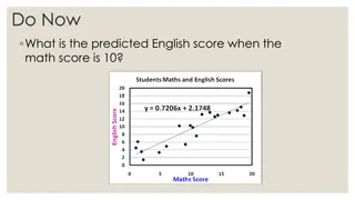
Scatterplots These are graphs in the 2-dimensional X-Y plane. Each point is a case in the data set and is represented by an ordered pair (X, Y), where X is its value for the predictor variable and Y is its value for the outcome variable. Are these points sort of in a line? (NOT a hump, U-shape, funnel, big shapeless cloud)
Line and not to be filled in Height and weight line for 180 students Something unlinear
Scatterplot (continued) If the answer is no, all is not lost, and we may be able to fix matters with a log transformation (see next slide). If the answer is yes, we can go ahead and build our linear model.
The log transformation for positively skewed variables If we see humps and funnels, we are often looking at skewed variables. If they are positively skewed, we can log- transform them, converting each numerical value to its log base e (e is an irrational number, close to 2.71). We can do this with a simple operation in the software. The logged variable will be near-normal and better to use in linear models.
The correlation coefficient, r If our variables are near-normal, we can compute the Pearson correlation coefficient r. It is a number that expresses the strength and direction (positive or negative) of the relationship of the two variables. It has a range between -1 and +1. -1 means a strong negative relationship; +1 means a strong positive relationship; 0 means no relationship at all.
Formula for r The formula: r = (Zx Zy)/N This is the average product-moment formula for r. For each case in the distribution, we multiply its Z- score for the X component by its Z-score for the Y component. We add up these products (one product for each case). We find the mean ( average ) for all the products by dividing by the number of cases.
Formula for r (continued) Notice that if the values for the variables are similar (high goes with high, low with low), r will be large and positive. Positive Z-scores go together, and negative Z- scores go together (height and weight) If the values for the variables are the inverse of each other (high on one goes with low on the other, low on one goes with high on the other), r will be large in absolute value and negative. Each case has a positive Z- score for one variable multiplied by a negative Z-score for the other variable (car weight and gas mileage).
Formula for r (continued) When we obtain the correlation coefficient for two variables, we can not only see whether it is close to +1 or -1, we can also see if it is statistically significant. When r is close to 0, it is more likely to NOT be statistically significant.
R-squared: the coefficient of determination R-squared will always be a value between 0 and +1. It can be read as a proportion and converted into a percentage (move the decimal point two spaces to the right). It is a way of answering the question: How good is our linear model?
How do we find R-squared? Shortcut: square r. How it really works: R-squared is calculated as the ratio of two variances: regression variance to total variance. Regression variance: A good variance based on the squared sum of the differences between the mean of the Y- distribution and the estimates in our model. Residual variance: A bad variance based on the (squared sum of the) differences between our estimated Y in the model and the real Y (the actually OBSERVED Y). Total variance: based on the (squared sum of the) differences between each observed Y and the mean of the Y distribution.
R-squared visualized If you think about the scatterplot and the regression line drawn through the dots, you can visualize R- squared. We would get a high value for R-squared if all the dots are close to the line we can do a good job drawing a line through our observed data points (the ordered pairs). R-squared has a low value if many of the points are far from the line. The residuals (distance of the Y component from the line) are large our estimated Y is generally not close to our observed Y.
Two slides: high and low R-squared In the next slides, we show a small segment of the calculation of R-squared: A regression line (sloping black line) with the estimated Y on it (black points). The observed (real data) Y points in red. The residuals are the distances between the estimated Y (black points) and the observed Y (red points). They are shown as orange lines.
R-squared visualization: good The next two slides help visualize R-squared. The first slide shows a GOOD situation. The estimated Y (in the regression model) is on the regression line (black point). The matching observed Y (real data) is the red point. The observed Y is consistently close to the estimated Y (in the text the estimated Y is Y-hat, but we can also use Y ).
Good: the residuals are small, and R- squared is large
R-squared visualization (continued) The next slide shows a BAD situation, in which the estimated Y in the regression model is usually not at all near the observed Y in the data. The distance between estimated Y and observed Y is large for most cases (orange lines). The residuals are LARGE, and so R-squared is small. Not very much of the total variance (based on the difference between observed-Y and the mean of the Y-distribution) is accounted for by the regression variance.
Bad: the residuals are large, and R- squared is small
R-squared: the end In the good case, the estimated Y on the regression line accounts for most of the variance of observed Y from the mean of the Y-distribution. R-squared is close to 1. In the bad case, the estimated Y on the regression line accounts for very little of the variance of Y from the mean of the Y- distribution. R-squared is low, near 0.
The Regression Model: the line The regression line that we are talking about is the Ordinary Least Squares line. It is a line whose slope we find by minimizing all the squared distances between the Y on the regression line and the observed Y (calculus problem). So it is the best fit line we can draw through all of our data points.
Coefficients of the Regression Line This line has the formula: Y = a + bX In the equation, b is the slope coefficient. The term a, the constant term, sometimes does not have much real world meaning: what would be my weight if I were 0 meters tall? The slope coefficient is tested for statistical significance. Null hypothesis: b = 0.
First: the slope coefficient The slope coefficient is calculated as the covariance of X and Y divided by the variance of X. This makes sense as rise over run how much do X and Y vary together for every unit of change in X? Notice it makes a difference which variable is the predictor variable. If we flip them, the slope coefficient will be different. (That is why Y comes first in the subscript of b.)
Summary and Key Terms Regression model, linear model, ordinary least squares line. Scatterplot, ordered pairs, best-fit line through the points. Log-transformation to make positively skewed variables near-normal. Correlation coefficient. Coefficient of determination, R-squared, ratio of regression variance to total variance. Coefficients of the regression line: slope coefficient and constant term. Slope coefficient: covariance divided by variance of X.


")


")
")


")