Comparison of Measurement Results for Tau Decay Time
The data provided includes measurements of tau (τ) decay time, resulting in half-lives (T½). Measurement 1 shows τ as 1.2 ps, converting to T½=0.83 ps, while Measurement 2 indicates T½=0.90 ps. The discrepancy between the two measurements prompts a closer examination of the experimental setup or analysis methods.

Download Presentation

Please find below an Image/Link to download the presentation.
The content on the website is provided AS IS for your information and personal use only. It may not be sold, licensed, or shared on other websites without obtaining consent from the author. Download presentation by click this link. If you encounter any issues during the download, it is possible that the publisher has removed the file from their server.
E N D
Presentation Transcript
Miscellaneous Problems Encountered in Mass Chain Reviews Murray Martin Oak Ridge national laboratory April, 2015
1. Available data: Example 1: Measurement 1: Measurement 2: =1.2 ps 2 which converts to T =0.83 ps 14 T = 0.90 ps 14 A weighted average of these two T values is 0.865 ps 99 or 0.86 ps 10 The evaluator converted to T and rounded it off to 0.8 ps 1, This results in a weighted average of 0.83 ps 8 By rounding off the value from , and rounding the uncertainty down, too much weight is given to that value, and the uncertainty in the average is too small.
2. In giving keynumbers, it is important to weed out unnecessary and superseded entries. Example 1. In a case where data from the same group are reported in more than one source, for example three primary sources with keynumbers A, B, and C, where A is the earliest and contains all the relevant material, the source should be stated as From A. Some (or all) of the data are also reported in B, and C . By expressing the comment in this way the readers are told that they need to look only at one reference, namely A. Even though there is nothing additional in the later references, it is important to include them in the comment so that readers will know that you were aware of them so they will not have to waste time tracking them down thinking they may contain new data. Example 2. In a case where a reference C supercedes earlier reports A, and B, by the same group, it is best to state this relationship as a comment on C rather than put A and B as Others: . The Others: category should be reserved for independent work Example 3. The ID record should not contain redundant entries. In example 1, only A should be given on the ID record. Similarly for example 2, only C should appear on the ID record. The others can be given as comments. 3.
3. Be aware of the interrelation between quantities in different datasets and the consequences of changes made in one or more of these quantities. Example 1 A decay scheme was normalized using as one piece of data the parent spin stated to be 3+. That spin was later changed to 1+; however, the normalization was not changed. Also, the J assignments that relied on J of the parent needed to be modified. Example 2: In dataset A, the relative order of the cascade 1- 2 from the E3 level was not established. The authors chose one ordering to establish a tentative intermediate E1 level. The relative order was later established in dataset B as reversed from that in A giving a level at E2. In dataset A the evaluator should delete level E1 and add level E2 with a comment on E2 stating something like A propose a level at E1 based on the 1- 2 cascade from level E3. The reverse order of the cascade is established in B, giving a level at E2 rather than at E1 .
4. Miscellaneous error: In a Coulomb Excitation dataset there were three keynumbers used in connection with BE2 for the first 2+ state. I label these keynumbers A, B, and C. 1. B and C are from the same group; however, the value from keynumber C was quoted with a smaller uncertainty than the value from B and yet was put as Others with no explanation. It turned out that reference C was an earlier report of the work quoted by B and in the evaluators judgement the later value should be the one adopted. A comment to this effect cleared up this point but this illustrates how important it is to explain choices that might be questioned. We are then left with data from references A and B. 2. The value from B was an absolute measurement. The value from A was stated as being relative to BE2=0.160 from reference D for a nuclide in another mass chain, M, but no uncertainty was included. I thought it worthwhile to see if there was an uncertainty associated with this reference value. The situation turned out to be rather complex and uncovered a problem in the way the data from D had been handled in mass chain M and also in reference A. Reference D quotes two measurements for the first 2+ state, =5.3 ps 3 from DSA and BE2=0.160 15. This BE2 value is the basis for the reference value quoted by A who apparently ignored the halflife measurement. The value of converts to T =3.67 ps 21, or BE2=0.142 8, and conversely BE2=0.160 15 converts to 3.26 ps 31. Problem #1: Problem #2: A references only the BE2 value from D. M adopted T =3.7 ps 2 from , but did not include enough digits, and moreover, the BE2 value from D was converted to T =3.3 ps 3 and given as Others:, so no use was made of what is really a comparably precise value and no mention was made that it came from a BE2 measurement. The recommended approach here would be to average the two BE2 values from D, pointing out that one measurement comes from T , and to correct the BE2 value given by A for this improved reference value. This average gives BE2= 0.148 7 or T =3.67 ps 18. The value from A can then be corrected for this improved reference value and averaged with the value from B. Finally, T =3.67 ps 18 should have been the value adopted in M.
5. Watch for obvious misprints in authors works. In a certain dataset, the uncertainties in I were all in the range of 12-15% except for one transition given as I =84 1. This uncertainty is clearly a misprint and should probably have been 10. It is recommended that the authors uncertainty be replaced and a comment given to state what was done.
6. 6. The usual propagation of errors formulae, based on a first order Taylor series expansion, are valid only for reasonably small fractional uncertainties. The deviation from validity depends on The usual propagation of errors formulae, based on a first order Taylor series expansion, are valid only for reasonably small fractional uncertainties. The deviation from validity depends on the operation being performed. the operation being performed. Example 1: When a quantity is squared, the fractional uncertainty in the product, to first order, is twice the fractional uncertainty in the original value, thus (3.0 1)2 becomes 9.0 0.6; however, (3.0 15) becomes 9 9, which overlaps zero, and (3.0 20)2 becomes 9 12, which allows the square quantity to be negative. An example of this problem occurred in a Coulomb excitation dataset in a mass chain on which I was working. The authors quoted only the matrix element. Extraction of BE2 then required squaring this matrix element. One such matrix element was quoted as 17.1 +62-96 eb. If one squares this and uses the uncertainty relation above, one gets BE2=6.5 +47-73, that is, the lower limit gives a negative BE2. This is non physical. BE2=6.5 +47-73, that is, the lower limit gives a negative BE2. This is non physical. Example 1: When a quantity is squared, the fractional uncertainty in the product, to first order, is twice the fractional uncertainty in the original value, thus (3.0 1)2 becomes 9.0 0.6; however, (3.0 15) becomes 9 9, which overlaps zero, and (3.0 20)2 becomes 9 12, which allows the square quantity to be negative. An example of this problem occurred in a Coulomb excitation dataset in a mass chain on which I was working. The authors quoted only the matrix element. Extraction of BE2 then required squaring this matrix element. One such matrix element was quoted as 17.1 +62-96 eb. If one squares this and uses the uncertainty relation above, one gets Uncertainty and range in x2 Uncertainty and range in x2 x x first order 2x x first order 2x x second order term=( x)2 second order term=( x)2 (x- x)2 x2 (x+ x)2 (x- x)2 x2 (x+ x)2 3.0 0.2 3.0 0.2 9.0 1.2 7.8 to 10.2 7.8 to 10.2 9.0 1.2 9.0 + 1.3 - 1.2 9.0 + 1.3 - 1.2 7.84 to 10.24 7.84 to 10.24 0.04 0.04 3.0 1.0 3.0 1.0 9.0 6.0 3.0 to 15.0 3.0 to 15.0 9.0 6.0 9.0 + 7.0 - 5.0 4.0 to 16.0 4.0 to 16.0 9.0 + 7.0 - 5.0 1.0 1.0 3.0 1.5 3.0 1.5 9.0 9.0 9.0 9.0 0 to 18.0 0 to 18.0 9.0 + 11 - 7 2.25 to 20.25 2.25 to 20.25 9.0 + 11 - 7 2.25 2.25 3.0 2.0 3.0 2.0 9.0 12.0 -3.0 to 21.0 -3.0 to 21.0 9.0 12.0 9.0 + 12.0 - 8.0 1.0 to 25.0 1.0 to 25.0 9.0 + 12.0 - 8.0 4.0 4.0 As shown in the table, when a quantity is squared, the uncertainty range correct to second order in a Taylor series expansion can be obtained simply by squaring the upper and lower bounds of the value. When applied to the actual case described above, one gets BE2=6.5 +56-53. the value. When applied to the actual case described above, one gets BE2=6.5 +56-53. As shown in the table, when a quantity is squared, the uncertainty range correct to second order in a Taylor series expansion can be obtained simply by squaring the upper and lower bounds of
Example 2: When faced with division, the second order terms in the Taylor series expansion are complex and for fractional uncertainties greater than about 10% lead to asymmetric values. The recommended approach in dealing with quantities appearing in the denominator of an equation is to take the reciprocal of the value at its upper and lower bounds. As an example, in calculating T from BE2, where T is inversely proportional to BE2, for a value of BE2= 0.25 0.5 one gets [BE2]-1 = 4.0 +1.0 - 0.7 and one can then proceed with the calculation. While this approach is probably not justified by a rigorous correct calculation, given the fact that we are usually dealing with uncertainties with unknown ratios of systematic to statistical components, which if known would require modification of all our formulae, this approach seems reasonable. Also, many of the uncertainties with which we deal are not rigorously assigned. Many authors state that their uncertainties are about 5% or that they range from 2% for the strong lines to 10% for the weak lines , without informing the reader what they mean by strong and weak.
8. Handling of discrepant gamma energies: In a case where an E is flagged in GTOL with five stars, indicating a deviation from the expected value of more than 5 , and if most of the other transitions fit well in the level scheme, I suggest not including that transition in the least-squares fit. One way to exclude this transition is to put a ? in column 80, then run GTOL, and then remove the ? . Apart from an outright mistake on the part of the author, a common reason for this poor fit to occur is when a peak is part of an unresolved or a poorly resolved multiplet. or of course if the transition has been misassigned to that level. If E (in) is the discrepant value, and E (out) is the value given by GTOL when the transition is excluded from the run, then I suggest entering a rounded-off E (out) value in the energy field, with no uncertainty, and giving a comment stating something like Rounded-off value from the least-squares adjustment, which gives E =E (out). The authors value of E =E (in) is a poor fit and is not included in the adjustment .
9. Rounding-off policies: Uncertainties: A decision has to be made as to when uncertainties should be rounded up. Most evaluators would agree that an uncertainty of 0.175 should be rounded up to 0.18, not down to 0.17, but where should this roundoff begin? My policy is to round up whenever the relevant digit in the uncertainty is 3 or higher. For example, I would round an uncertainty of 0.173 to 0.18. We have no set policy on this matter in the Network, and perhaps some evaluators would choose a different cutoff. Perhaps we could agree on a cutoff and make it a policy. I feel that it is better to overstate an uncertainty than to understate it. Rounding of numbers ending in 5": It is the usual practice in numerical analysis, when rounding a final digit, to round up odd digits but not even digits, thus 25" rounds to 2" while 55" rounds to 6". The reason usually given for this policy is that in cases where one is averaging a set of values, this procedure avoids biasing the answer either up or down. This is not a stated policy of the Network, but as mentioned it is a standard practice in numerical analysis. I believe nearly all evaluators use this policy.
10. Miscellaneous: Branching in Adopted Gammas In adopted gammas, for a level with just two deexciting transitions the best way to get the adopted branching is to simply average the ratios from the individual sets of measurements. This works as long as one doesn t have to divide by a value with a large fractional uncertainty. When this is done, the stronger transition can be assigned I =100 with or without an uncertainty. If an uncertainty is assigned to the value 100", then that fractional uncertainty must be subtracted in quadrature from the intensity of the weaker component. There is usually no reason to assign an uncertainty to the normalization transition in such cases since the important quantity is just the ratio. As an example, consider three measurements of I (A)/I (B), namely 0.326 21, 0.314 14, and 0.318 18 whose weighted average is 0.318 10. One can then adopt I (A)=31.8 10 with I (B)=100 or, if the smallest uncertainty in I (B) among the three measurements has an uncertainty of 2% and one wants to show this, one can adopt 31.8 8 and 100 2. The first approach is preferable since it avoids any additional roundoff.
11. Miscellaneous: Asymmetric (exp): In cases where mult and come from (exp), then the experimental value of is what should be entered in the CC field. A problem occurs when (exp) is asymmetric since we can t use asymmetric uncertainties for that field. In such a case the best one can do is to adopt a symmetrized value and give the original value in a comment. Of course this value of will no longer be consistent with the entered in the MR field so one will need to add a comment stating that is deduced from the experimental asymmetrical value.
12. Miscellaneous: problem in averaging. Reference A reported two values of a halflife, 478 ms 44 and 495 ms 60. The evaluator took the average of these two values as given by the authors, namely 484 35 and then averaged that value with 485 40 from a second reference. The result is 484 26, the same result that one gets by taking an average of all three values, as expected; however, the evaluator then stated that rather than adopting the uncertainty from the weighted average, he/she had adopted the smallest measured uncertainty. The value so chosen was 35", the uncertainty from the first average. The correct value using the stated criterion should have been the smallest uncertainty for the three independent values, namely 40, rather than 35.
13. Asymmetric uncertainties in averages: The network has no guidelines on how to handle asymmetric uncertainties when taking averages. Consider a case where one has input values of 0.087 ps +28-21 and 0.10 3. A reasonable approach in this case might be to calculate the average using the upper uncertainty, 0.093 20, and that using the lower uncertainty, 0.091 17 and combine them to get 0.092 +21-16. I ve chosen a case here where the difference in the upper and lower values is small, and this is often the case. If the difference is large, perhaps quoting both upper and lower values would be useful Perhaps someone in the audience has a suggestion and would be willing to write up a procedure for this situation.
14. J arguments: 1. All arguments used to establish J for an adopted level should be traceable back to the source dataset. If the J argument includes L(d,p)=1 from 1/2+ then the (d,p) dataset should show L=1 for that level. If an argument states M1 to 5/2- , then the transition in question should be shown as M1 in adopted gammas with the justification for that assignment clearly stated. If the argument states J =2- is ruled out from excit in ( .xn ) , then the source dataset should back up this statement. As a corollary to this approach, do not put the justifications for the L assignment or the mult assignment in with the J argument. That is, do not state something like L(d,p)=1 from 1/2+ based on ( ) and a DWBA fit . Doing this makes the J arguments much harder to read. Leave the details to the source dataset. The fact that an evaluator uses L=1 implies that he/she has been convinced of its reliability. 2. It can be useful in some cases to give a J argument even when no J is assigned. It may be known that a level decays to a 2+ level. which usually justifies assuming that J lies in the range 0 to 4. This range exceeds our recommended range limit of three values for inclusion an the J field; however, by giving this J argument the reader knows that J cannot be high spin, and in a nuclide with a lot of high spin data, this may be a useful piece of data. As recommended elsewhere for other situations, it is perhaps best to use a flagged footnote for such an argument. This puts a flag in the J field and is more likely to catch a reader s attention than would be a comment.
15. Corrections for misprints, typos etc., and recalibrations: Whenever a value is corrected, whether it be a typo on the part of the authors or a correction applied by the evaluator as a result of newer calibration standards, the corrected value should be put in the relevant field and the original value put in a comment. Do not put the original value in the field and rely on a comment to convey the corrected value.
16. An attempt should be made to resolve discrepancies among datasets. Example 1: A level at 2307 is proposed in three experiments. The 921 is not reported in +, but there is a peak in the spectrum that is consistent with a transition at this energy with an intensity reasonably close (within a factor of 2) to that of the 1692 . The + and (p,n ) data are thus reasonably consistent, but neither reports the 1279 . The 1279 reported in (p, ) clearly does not belong with the 2307 level seen in the other two works. Also, I (920 ) in (p, ) is too large, indicating that a large fraction of its intensity must belong elsewhere. It is possible that the excess intensity of the 920 and the 1279 could together define a close-lying doublet at 2307. (p, ) + (p,n ) E I E I E I 100 920.3 455 921? 920.6 85 (4) 1279.0 123 1691.7 100 1692.0 (15) 100 1692.0 100 (4)
Example 2: In a case where you have three or more transitions from a level and more than two measurements of the branching ratios from that level, if two of them agree but the third differs significantly, it may be possible to say something useful about the discrepant value. E I A B C 100 100 100 1 82 2 79 3 83 3 2 57 3 55 4 78 3 3 18 1 21 2 19 3 4 From these data it would be reasonable to conclude that in source C, the transition 3 is multiply placed, with only part of its intensity belonging with the level in question.
17. T (252Cf): The following is a listing of all comparably precise measurements for the halflife of 252Cf and how they were treated by four evaluations in orderv to arrive at a recommended value. Reference Value (y) A (1986) B (2008) C (2006) D (1992) 1965Me02 2.646 4 Y Y Y Y X1969De23 2.621 6 Y Y 1 Y Y 1973Mi05 2.659 10 Y Y 1 Y Y X1974Sh15 2.628 10 Y Y 2 Y Y 2 X1974Sp02 2.638 7 N 3 Y Y N 1976Mo30 2.637 5 Y Y Y Y Alberts *(1980) 2.648 2 Y Y Y Y Spiegel* (1980) 2.653 1 Y N Y N 1982La25 2.639 7 Y Y Y Y 1984SmZV 2.651 3 Y Y Y Y 1985Ax02 2.6503 31 Y Y Y N 1992Sh33 2.645 3 N Y Y N Recommendations 2.6501 17 Weighted average of all data except value of 1974Sp02. 2.6505 13 Weighted average of all data except values of 1974Sp02 and 1969De23 (ruled an outlier by Chauvenet s criterion) 2.6470 14 Weighted average from B of all data except 1974Sp02 and Spiegel (not considered by B) and both 1969De23 and 1973Mi05, considered by them as outliers. 2.6470 26 Value recommended by B with uncertainty of 0.1% applied to account for possible systematic uncertainties 2.6505 26 or 2.650 3 PC to A Rejected by Chauvenet s criterion in C Superseded by 1992Sh33 Value subsequently withdrawn by authors according to A Value recommended by present evaluator with uncertainty of 0.1% assigned as recommended by B. Keynumbers marked with X are not included * 1 2 3
Miscellaneous: energies and intensities: Unless an endpoint energy is of a quality high enough to be included in the mass adjustment, it is recommended that they be put in comments. Note that all the Network programs that require E will calculate that quantity from the Q value and the level energy. If poorly measured endpoint energies are entered into the energy field for a decay where the Q value and daughter level energies are accurately known one can end up with endpoint energies in the table and in the drawing being out of order. In general. the IB field values deduced from the I( +ce) imbalances should always be those of the evaluator. Note that in the general case the evaluator might have some different gamma mult assignments from those of the authors, and the gamma intensities might be averages from several sources. The I( -) values follow directly from the I and data (or TI) given in your gamma listing, so all that is needed is a comment on I( -) or I( + + ) stating From an intensity balance at each level . An exception would be a case where the I for one or more branches were used to normalize the decay scheme. Intensities for such branches should be entered in the IB field.